
A good number needs a good question.
Explore 32 decision labs spanning measurement, error correction, networking, control and sensing. Compare complete input regimes, follow the calculation and discover which assumption changes the answer.
Evidence and experimental design
Evidence and experimental designA fair control experiment can start with the pairingWhat changes when two implementations experience the same batch disturbance?
Imagine comparing two pulse implementations during a day when a laboratory drifts between warmer and cooler operating conditions. Running all of A first and all of B later confounds implementation with time. Even if the total number of shots is large, a difference between the batches can masquerade as a difference between the methods. The experimental unit must be identified before the error bar is chosen.
A matched design asks A and B to encounter similar conditions and records their difference within each match. A disturbance shared by both measurements can then cancel. The relevant variation is the variation of the differences, rather than the sum of two variances treated as unrelated. Pairing earns this benefit only when the correspondence is real. Pairing unrelated records after inspecting their outcomes is not the same experiment.
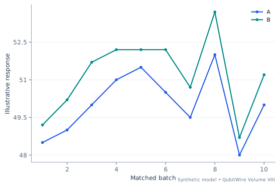
This laboratory constructs ten matched batches with a shared disturbance and smaller difference noise. Its calculation shows the exact standard-error consequence of retaining or discarding the match. The learning goal is to ask what was randomized, what was repeated, and which conditions were shared. A quantum benchmark can have thousands of circuit shots while still having very few independent calibration batches.
Start with the assumptions
- Each pair shares the declared disturbance.
- Difference-noise values are constructed, not sampled from a fitted distribution.
- The sample standard deviation uses denominator n - 1.
d_i = B_i - A_i; mean difference = sum(d_i)/n
SE_paired = sample_SD(d)/sqrt(n)
SE_unpaired = sqrt(sample_Var(A)/n + sample_Var(B)/n)
Compare the input regimes
Each case uses invented inputs. The results follow from this model and do not describe measured hardware.
Baseline regime
Complete inputs
- Common disturbance scale
- 0.5
- Difference noise scale
- 0.5
- True shift
- 1.2
- Response baseline
- 50
- Shared disturbance pattern
- -3, -2, 0, 2, 3, 1, -1, 4, -4, 0
- Difference-noise pattern
- -1, 0, 1, 0, -1, 1, 0, 1, -1, 0
- Compute ten matched differences B_i - A_i. Their mean is 1.2 and their sample standard deviation is 0.408248.
- Divide the difference standard deviation by sqrt(10), giving 0.129099. Treating the same observations as unpaired gives 0.632456.
- The paired calculation retains the shared disturbance as covariance; it cancels in each difference. The unpaired expression discards that relationship.
| Calculated quantity | Synthetic result |
|---|---|
| Batch pairs | 10 |
| Mean B minus A | 1.2000000000000028 |
| Paired standard error | 0.12909944487358055 |
| Unpaired standard error | 0.6324555320336759 |
| Unpaired / paired variance | 24.000000000000004 |
| Pair | A | B | B − A |
|---|---|---|---|
| 1 | 48.5 | 49.2 | 0.7000000000000028 |
| 2 | 49 | 50.2 | 1.2000000000000028 |
| 3 | 50 | 51.7 | 1.7000000000000028 |
| 4 | 51 | 52.2 | 1.2000000000000028 |
| 5 | 51.5 | 52.2 | 0.7000000000000028 |
| 6 | 50.5 | 52.2 | 1.7000000000000028 |
| 7 | 49.5 | 50.7 | 1.2000000000000028 |
| 8 | 52 | 53.7 | 1.7000000000000028 |
| 9 | 48 | 48.7 | 0.7000000000000028 |
| 10 | 50 | 51.2 | 1.2000000000000028 |
The variance ratio is 24 in this constructed batch. Matching is useful because the common disturbance is genuinely shared. These ten deliberately chosen observations do not validate a population distribution or establish a significance level.
Comparison regime
Complete inputs
- Common disturbance scale
- 2
- Difference noise scale
- 0.62
- True shift
- 1.95
- Response baseline
- 50
- Shared disturbance pattern
- -3, -2, 0, 2, 3, 1, -1, 4, -4, 0
- Difference-noise pattern
- -1, 0, 1, 0, -1, 1, 0, 1, -1, 0
- Compute ten matched differences B_i - A_i. Their mean is 1.95 and their sample standard deviation is 0.506228.
- Divide the difference standard deviation by sqrt(10), giving 0.160083. Treating the same observations as unpaired gives 2.367902.
- The paired calculation retains the shared disturbance as covariance; it cancels in each difference. The unpaired expression discards that relationship.
| Calculated quantity | Synthetic result |
|---|---|
| Batch pairs | 10 |
| Mean B minus A | 1.9500000000000028 |
| Paired standard error | 0.16008331164323922 |
| Unpaired standard error | 2.36790202500019 |
| Unpaired / paired variance | 218.79396462018917 |
| Pair | A | B | B − A |
|---|---|---|---|
| 1 | 44 | 45.330000000000005 | 1.3300000000000054 |
| 2 | 46 | 47.95 | 1.9500000000000028 |
| 3 | 50 | 52.57 | 2.5700000000000003 |
| 4 | 54 | 55.95 | 1.9500000000000028 |
| 5 | 56 | 57.330000000000005 | 1.3300000000000054 |
| 6 | 52 | 54.57 | 2.5700000000000003 |
| 7 | 48 | 49.95 | 1.9500000000000028 |
| 8 | 58 | 60.57 | 2.5700000000000003 |
| 9 | 42 | 43.330000000000005 | 1.3300000000000054 |
| 10 | 50 | 51.95 | 1.9500000000000028 |
The variance ratio is 218.793965 in this constructed batch. Matching is useful because the common disturbance is genuinely shared. These ten deliberately chosen observations do not validate a population distribution or establish a significance level.
Extended regime
Complete inputs
- Common disturbance scale
- 3.8
- Difference noise scale
- 0.86
- True shift
- 2.8499999999999996
- Response baseline
- 50
- Shared disturbance pattern
- -3, -2, 0, 2, 3, 1, -1, 4, -4, 0
- Difference-noise pattern
- -1, 0, 1, 0, -1, 1, 0, 1, -1, 0
- Compute ten matched differences B_i - A_i. Their mean is 2.85 and their sample standard deviation is 0.702187.
- Divide the difference standard deviation by sqrt(10), giving 0.222051. Treating the same observations as unpaired gives 4.467241.
- The paired calculation retains the shared disturbance as covariance; it cancels in each difference. The unpaired expression discards that relationship.
| Calculated quantity | Synthetic result |
|---|---|
| Batch pairs | 10 |
| Mean B minus A | 2.8500000000000005 |
| Paired standard error | 0.2220510451825581 |
| Unpaired standard error | 4.467240759126376 |
| Unpaired / paired variance | 404.73715521903904 |
| Pair | A | B | B − A |
|---|---|---|---|
| 1 | 38.6 | 40.59 | 1.990000000000002 |
| 2 | 42.4 | 45.25 | 2.8500000000000014 |
| 3 | 50 | 53.71 | 3.710000000000001 |
| 4 | 57.6 | 60.45 | 2.8500000000000014 |
| 5 | 61.4 | 63.39 | 1.990000000000002 |
| 6 | 53.8 | 57.51 | 3.710000000000001 |
| 7 | 46.2 | 49.050000000000004 | 2.8500000000000014 |
| 8 | 65.2 | 68.91 | 3.7099999999999937 |
| 9 | 34.8 | 36.79 | 1.990000000000002 |
| 10 | 50 | 52.85 | 2.8500000000000014 |
The variance ratio is 404.737155 in this constructed batch. Matching is useful because the common disturbance is genuinely shared. These ten deliberately chosen observations do not validate a population distribution or establish a significance level.
Try the reasoning: Before calculating an error bar, identify the independent experimental unit. What evidence justifies the correspondence within each pair?
Sources and model boundaries
- Two-Sample t-Test for Equal Means ↗
A paired comparison has a one-to-one correspondence between observations, allowing analysis of within-pair differences. The lab does not reuse NIST data or claim a significance test for its deterministic records.
- Combining uncertainty components ↗
Uncertainty propagation includes sensitivities and covariance; independent terms simplify the variance sum. Covariance, bias and distribution assumptions in the teaching models are declared separately; no NIST endorsement is implied.
Evidence and experimental designA better result in every workload can lose the combined scoreCan a changing workload mix reverse a performance comparison?
A benchmark suite is a distribution of questions. If a provider runs mostly easy instances while another tackles mostly hard ones, their overall completion percentages answer different questions. Neither percentage is wrong as a description of its own workload. The mistake occurs when the two denominators are treated as interchangeable evidence about the methods.
The constructed example contains only two strata, easy and hard. Method B improves the stipulated success probability in both. It is nevertheless possible to make B look worse overall by allocating more hard work to B. The reversal comes entirely from the weights. There is no hidden quantum effect and no arithmetic paradox once those weights become visible.
Standardization chooses one reference workload and evaluates both methods against it. That requires a defensible reference: the published challenge set, a fixed deployment distribution or a clearly labeled teaching mixture. A fair comparison keeps both the observed mix and the standardized comparison. Discarding the operational mix can erase useful information about what a service actually handled; discarding standardization can reward an easier test.
Start with the assumptions
- Within-stratum rates are known synthetic probabilities.
- Easy and hard are fixed categories with comparable meanings.
- No uncertainty intervals are attached to stipulated rates.
Mixed success = easy_fraction × p_easy + (1-easy_fraction) × p_hard
Standardized success uses the same easy_fraction for both methods
Percentage-point difference = 100 × (p_B - p_A)
Compare the input regimes
Each case uses invented inputs. The results follow from this model and do not describe measured hardware.
Baseline regime
Complete inputs
- A easy success
- 0.93
- A hard success
- 0.47
- B within-stratum gain
- 0.02
- A easy workload fraction
- 0.55
- B easy workload fraction
- 0.4
- Reference easy fraction
- 0.2
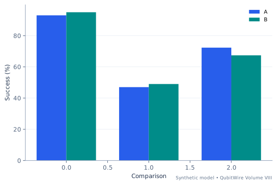
- A is weighted using 55% easy work; B uses 40%. Those are different test distributions.
- Use the shared 20% easy reference for both: A = 0.562, B = 0.582.
- The raw difference is -4.9 percentage points. The shared-workload difference is 2 percentage points.
| Calculated quantity | Synthetic result |
|---|---|
| A mixed success (%) | 72.30000000000001 |
| B mixed success (%) | 67.4 |
| Raw B minus A (percentage points) | -4.900000000000004 |
| A standardized success (%) | 56.2 |
| B standardized success (%) | 58.20000000000001 |
| Standardized gain (percentage points) | 2.0000000000000018 |
The direction reverses after standardization. B was defined to improve both strata by 2 percentage points. Aggregation cannot identify that fact without the workload mix. These rates are stipulated probabilities, not estimates with sampling intervals.
Comparison regime
Complete inputs
- A easy success
- 0.93
- A hard success
- 0.47
- B within-stratum gain
- 0.03
- A easy workload fraction
- 0.7000000000000001
- B easy workload fraction
- 0.325
- Reference easy fraction
- 0.45
- A is weighted using 70% easy work; B uses 32.5%. Those are different test distributions.
- Use the shared 45% easy reference for both: A = 0.677, B = 0.707.
- The raw difference is -14.25 percentage points. The shared-workload difference is 3 percentage points.
| Calculated quantity | Synthetic result |
|---|---|
| A mixed success (%) | 79.2 |
| B mixed success (%) | 64.95 |
| Raw B minus A (percentage points) | -14.249999999999996 |
| A standardized success (%) | 67.7 |
| B standardized success (%) | 70.7 |
| Standardized gain (percentage points) | 3.0000000000000027 |
The direction reverses after standardization. B was defined to improve both strata by 3 percentage points. Aggregation cannot identify that fact without the workload mix. These rates are stipulated probabilities, not estimates with sampling intervals.
Extended regime
Complete inputs
- A easy success
- 0.93
- A hard success
- 0.47
- B within-stratum gain
- 0.041999999999999996
- A easy workload fraction
- 0.88
- B easy workload fraction
- 0.23500000000000004
- Reference easy fraction
- 0.75
- A is weighted using 88% easy work; B uses 23.5%. Those are different test distributions.
- Use the shared 75% easy reference for both: A = 0.815, B = 0.857.
- The raw difference is -25.47 percentage points. The shared-workload difference is 4.2 percentage points.
| Calculated quantity | Synthetic result |
|---|---|
| A mixed success (%) | 87.48 |
| B mixed success (%) | 62.01000000000001 |
| Raw B minus A (percentage points) | -25.46999999999999 |
| A standardized success (%) | 81.5 |
| B standardized success (%) | 85.7 |
| Standardized gain (percentage points) | 4.200000000000015 |
The direction reverses after standardization. B was defined to improve both strata by 4.2 percentage points. Aggregation cannot identify that fact without the workload mix. These rates are stipulated probabilities, not estimates with sampling intervals.
Try the reasoning: Choose a second common workload distribution. Does the within-stratum improvement change, or only the aggregate score?
Evidence and experimental designA shot budget is also a time budgetHow should measurement effort change when groups take different amounts of time?
The most variable contribution to an observable may deserve extra measurement effort, but that is not the complete allocation question. Some settings take longer to prepare, some require a costly basis change, and others produce information much more cheaply. A fixed number of shots and a fixed amount of laboratory time impose different constraints.
This lab combines observable coefficients, group variances and per-shot time. The continuous calculation has a closed-form optimum under its assumptions. Converting it to integer shot counts then introduces a small implementation problem: rounding can waste time or slightly change the optimum. The worked answers expose both the lower bound and the rounded schedule instead of hiding the distinction behind an allocation score.
The model assumes the groups are independently estimated and their variances are known. A real pilot experiment spends part of the budget learning those variances. Calibration and circuit switching may add costs that depend on how measurements are grouped. Increasing one time cost while holding its physical variance fixed changes the preferred allocation. The resource tradeoff is conditional on these assumptions; different Hamiltonians and acquisition workflows can require different schedules.
Start with the assumptions
- Group estimates are independent.
- Variances, coefficients and per-shot costs are known and stationary.
- The rounded greedy schedule is compared with a continuous bound, not certified as the integer optimum.
V = sum_i (a_i sigma_i)^2 / n_i; sum_i c_i n_i <= T
n_i* = T |a_i| sigma_i / (sqrt(c_i) sum_j |a_j| sigma_j sqrt(c_j))
Continuous lower bound V* = (sum_i |a_i| sigma_i sqrt(c_i))² / T
Compare the input regimes
Each case uses invented inputs. The results follow from this model and do not describe measured hardware.
Baseline regime
Complete inputs
- Time costs per shot
- 1, 2, 5
- Group standard deviations
- 1, 1.4, 0.6
- Observable coefficients
- 1, -0.5, 1.2
- Time budget
- 1200
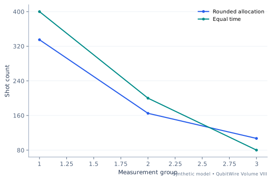
- The continuous solution allocates 333.340886, 164.99532, 107.333695 shots. It minimizes variance under the time constraint before integer rounding.
- Round down, then spend affordable remaining units by the largest immediate variance reduction per unit time. The resulting counts are 335, 165, 107. This greedy rounding is not claimed to solve every integer allocation problem exactly.
- Variance is sum((coefficient × standard deviation)^2 / shots) = 0.0108. Equal time across groups yields 0.01143.
| Calculated quantity | Synthetic result |
|---|---|
| Allocated shots, group 1 | 335 |
| Allocated shots, group 2 | 165 |
| Allocated shots, group 3 | 107 |
| Used time | 1200 |
| Allocated variance | 0.010799631409646753 |
| Equal-time variance | 0.01143 |
| Continuous lower bound | 0.010799510630309797 |
| Group | Continuous shots | Rounded shots | Equal-time shots |
|---|---|---|---|
| 1 | 333.3408855913823 | 335 | 400 |
| 2 | 164.99532045387687 | 165 | 200 |
| 3 | 107.33369470017277 | 107 | 80 |
The rounded allocation uses 1,200 of 1,200 time units. Its variance is 0.001118% above the continuous lower bound. The calculation shows why a costly measurement may deserve fewer shots even when its contribution is noisy.
Comparison regime
Complete inputs
- Time costs per shot
- 1, 3, 7
- Group standard deviations
- 1, 1.7999999999999998, 0.8
- Observable coefficients
- 1, -0.5, 1.2
- Time budget
- 2700
- The continuous solution allocates 529.53979, 275.156946, 192.141339 shots. It minimizes variance under the time constraint before integer rounding.
- Round down, then spend affordable remaining units by the largest immediate variance reduction per unit time. The resulting counts are 531, 275, 192. This greedy rounding is not claimed to solve every integer allocation problem exactly.
- Variance is sum((coefficient × standard deviation)^2 / shots) = 0.009629. Equal time across groups yields 0.011011.
| Calculated quantity | Synthetic result |
|---|---|
| Allocated shots, group 1 | 531 |
| Allocated shots, group 2 | 275 |
| Allocated shots, group 3 | 192 |
| Used time | 2700 |
| Allocated variance | 0.009628693716829308 |
| Equal-time variance | 0.01101111111111111 |
| Continuous lower bound | 0.009628675841389512 |
| Group | Continuous shots | Rounded shots | Equal-time shots |
|---|---|---|---|
| 1 | 529.5397902499327 | 531 | 900 |
| 2 | 275.1569464026749 | 275 | 300 |
| 3 | 192.1413386488632 | 192 | 128 |
The rounded allocation uses 2,700 of 2,700 time units. Its variance is 0.000186% above the continuous lower bound. The calculation shows why a costly measurement may deserve fewer shots even when its contribution is noisy.
Extended regime
Complete inputs
- Time costs per shot
- 1, 5, 7
- Group standard deviations
- 1, 2.28, 1.04
- Observable coefficients
- 1, -0.5, 1.2
- Time budget
- 4500
- The continuous solution allocates 656.836967, 334.870921, 309.829776 shots. It minimizes variance under the time constraint before integer rounding.
- Round down, then spend affordable remaining units by the largest immediate variance reduction per unit time. The resulting counts are 662, 335, 309. This greedy rounding is not claimed to solve every integer allocation problem exactly.
- Variance is sum((coefficient × standard deviation)^2 / shots) = 0.01043. Equal time across groups yields 0.012277.
| Calculated quantity | Synthetic result |
|---|---|
| Allocated shots, group 1 | 662 |
| Allocated shots, group 2 | 335 |
| Allocated shots, group 3 | 309 |
| Used time | 4500 |
| Allocated variance | 0.010430443022618991 |
| Equal-time variance | 0.012276722741433023 |
| Continuous lower bound | 0.010430312959808825 |
| Group | Continuous shots | Rounded shots | Equal-time shots |
|---|---|---|---|
| 1 | 656.8369671128199 | 662 | 1500 |
| 2 | 334.8709207605855 | 335 | 300 |
| 3 | 309.8297755834646 | 309 | 214 |
The rounded allocation uses 4,500 of 4,500 time units. Its variance is 0.001247% above the continuous lower bound. The calculation shows why a costly measurement may deserve fewer shots even when its contribution is noisy.
Try the reasoning: Which group gains most from the next affordable shot? Compare its variance reduction per unit time with that of the other groups.
Sources and model boundaries
- Combining uncertainty components ↗
Uncertainty propagation includes sensitivities and covariance; independent terms simplify the variance sum. Covariance, bias and distribution assumptions in the teaching models are declared separately; no NIST endorsement is implied.
Evidence and experimental designCorrelated measurements can call for an unexpected weightWhen is averaging two estimates less useful than combining their shared noise explicitly?
Two instruments can agree because both see the same disturbance. Agreement then contains less independent information than it appears to. Conversely, carefully combining correlated signals can sometimes cancel a disturbance. The deciding object is the covariance matrix, which records how the errors move together as well as how large each error is.
For two unbiased estimates, any weights that sum to one preserve the common mean. The variance is a quadratic function of one remaining weight. Minimizing it can produce an ordinary weighted average or a coefficient outside the interval from zero to one. A negative weight subtracts a correlated contribution; it is not a negative probability. Such cancellation also makes the answer more dependent on the validity of the error model.
The cases compare three choices: equal weights, an independence-based weighting, and a covariance-aware weighting. All three are evaluated using the same actual covariance. That last step matters: an algorithm should not be rewarded by calculating its uncertainty under the very assumption being questioned. Varying the correlation while keeping both individual uncertainties fixed isolates the role of shared noise.
Start with the assumptions
- Both estimates are unbiased for the same quantity.
- The covariance matrix is positive definite in the tested regimes.
- Weights are chosen from known uncertainty inputs, not from favorable observed outcomes.
Var(wA+(1-w)B) = w² v_A + (1-w)² v_B + 2w(1-w)c
w* = (v_B-c)/(v_A+v_B-2c)
c = rho × s_A × s_B
Compare the input regimes
Each case uses invented inputs. The results follow from this model and do not describe measured hardware.
Baseline regime
Complete inputs
- Sensor A standard uncertainty
- 1
- Sensor B standard uncertainty
- 1.8
- Correlation
- -0.3
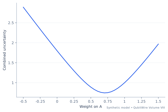
- Covariance = correlation × s_A × s_B = -0.54. Insert it in all three variance terms.
- Differentiate the variance with respect to A’s weight, with B’s weight fixed to 1 - w. The stationary point gives w = 0.710526.
- The standard uncertainty is sqrt(0.554211) = 0.744453. An independence-based weight is 0.764151, but its real variance must still include covariance.
| Calculated quantity | Synthetic result |
|---|---|
| Optimal A weight | 0.7105263157894737 |
| Optimal B weight | 0.2894736842105263 |
| Combined standard uncertainty | 0.74445317268166 |
| Equal-weight uncertainty | 0.8888194417315589 |
| Ignore-correlation weight, evaluated correctly | 0.7546580165645312 |
Both weights lie between zero and one in this regime. The estimate is unbiased only because both inputs were assumed unbiased and the weights sum to one. A gain error or wrong covariance can reverse this result.
Comparison regime
Complete inputs
- Sensor A standard uncertainty
- 1.25
- Sensor B standard uncertainty
- 2
- Correlation
- 0.2
- Covariance = correlation × s_A × s_B = 0.5. Insert it in all three variance terms.
- Differentiate the variance with respect to A’s weight, with B’s weight fixed to 1 - w. The stationary point gives w = 0.767123.
- The standard uncertainty is sqrt(1.315068) = 1.146764. An independence-based weight is 0.719101, but its real variance must still include covariance.
| Calculated quantity | Synthetic result |
|---|---|
| Optimal A weight | 0.7671232876712328 |
| Optimal B weight | 0.23287671232876717 |
| Combined standard uncertainty | 1.1467643581619917 |
| Equal-weight uncertainty | 1.2808688457449497 |
| Ignore-correlation weight, evaluated correctly | 1.1513427826920897 |
Both weights lie between zero and one in this regime. The estimate is unbiased only because both inputs were assumed unbiased and the weights sum to one. A gain error or wrong covariance can reverse this result.
Extended regime
Complete inputs
- Sensor A standard uncertainty
- 1.55
- Sensor B standard uncertainty
- 2
- Correlation
- 0.8
- Covariance = correlation × s_A × s_B = 2.48. Insert it in all three variance terms.
- Differentiate the variance with respect to A’s weight, with B’s weight fixed to 1 - w. The stationary point gives w = 1.053726.
- The standard uncertainty is sqrt(2.398336) = 1.548656. An independence-based weight is 0.624756, but its real variance must still include covariance.
| Calculated quantity | Synthetic result |
|---|---|
| Optimal A weight | 1.0537261698440212 |
| Optimal B weight | -0.05372616984402123 |
| Combined standard uncertainty | 1.5486562632931455 |
| Equal-weight uncertainty | 1.6854153790683175 |
| Ignore-correlation weight, evaluated correctly | 1.6321086060481949 |
The optimal solution uses a negative weight, which subtracts shared noise while increasing sensitivity to model error. The estimate is unbiased only because both inputs were assumed unbiased and the weights sum to one. A gain error or wrong covariance can reverse this result.
Try the reasoning: Find the regime with a weight outside zero to one. Which covariance assumption makes that subtraction useful, and which calibration error could invalidate it?
Sources and model boundaries
- Combining uncertainty components ↗
Uncertainty propagation includes sensitivities and covariance; independent terms simplify the variance sum. Covariance, bias and distribution assumptions in the teaching models are declared separately; no NIST endorsement is implied.
Evidence and experimental designOne campaign can ask enough questions to manufacture a surpriseHow does searching many comparisons change the chance of a false alert?
A benchmark campaign may compare dozens of circuits, calibrations, devices and parameter choices. Even if every individual statistical test has a small false-positive probability, the chance of at least one apparent surprise can become large. Selecting the most flattering comparison after the search conceals the size of that campaign.
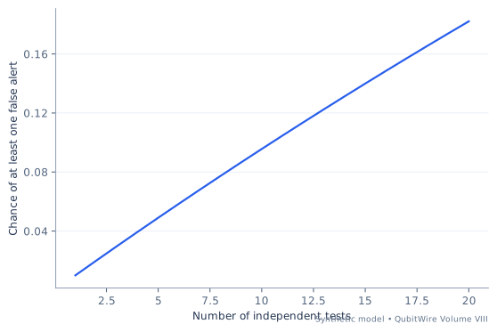
This lab assumes all tested null hypotheses are true and computes the exact independent-test probability of at least one false alert. It then introduces a simple family-wide bound by dividing the desired total error allowance among the tests. The exact probability uses independence. The union-bound guarantee does not, provided each individual false-positive bound is valid. Keeping those two claims separate is the main mathematical lesson.
A correction is not a complete scientific analysis. It can reduce the power to detect a real effect, and it does not repair data leakage, a biased estimator or an inappropriate null model. The number of comparisons therefore belongs in the experiment plan. Predeclared endpoints and a fresh validation set can make the campaign easier to interpret than a long list of selected p-values.
Start with the assumptions
- Every null hypothesis is true in this scenario.
- Exact family probabilities use independent tests.
- Each individual cutoff is a valid false-positive probability bound.
P(at least one false alert) = 1-(1-alpha)^m under independence
Expected number of false alerts = m alpha
Bonferroni per-test cutoff = desired_family_bound/m
Compare the input regimes
Each case uses invented inputs. The results follow from this model and do not describe measured hardware.
Baseline regime
Complete inputs
- Tests in campaign
- 20
- Per-test false-positive probability
- 0.01
- Desired family upper bound
- 0.05
- All 20 null hypotheses are assumed true. Independence gives the probability of no alert as (1 - 0.01)^20.
- Subtract from one: the campaign alert probability is 0.182093, even though each test uses 0.01.
- Dividing the desired family bound 0.05 by 20 gives 0.0025. The union bound does not require independent tests; the displayed exact corrected probability does.
| Calculated quantity | Synthetic result |
|---|---|
| Expected false alerts | 0.2 |
| Chance of one or more false alerts | 0.18209306240276915 |
| Bonferroni per-test cutoff | 0.0025 |
| Bonferroni family upper bound | 0.05 |
| Independent-test family probability after correction | 0.04883012474683423 |
At least one false alert occurs with probability 18.209306% under the independent all-null scenario. The correction is a declared campaign rule, not a substitute for replication or a complete analysis of statistical power. A laboratory must count the comparisons actually searched, including hidden tuning decisions.
Comparison regime
Complete inputs
- Tests in campaign
- 120
- Per-test false-positive probability
- 0.01
- Desired family upper bound
- 0.05
- All 120 null hypotheses are assumed true. Independence gives the probability of no alert as (1 - 0.01)^120.
- Subtract from one: the campaign alert probability is 0.70062, even though each test uses 0.01.
- Dividing the desired family bound 0.05 by 120 gives 0.000417. The union bound does not require independent tests; the displayed exact corrected probability does.
| Calculated quantity | Synthetic result |
|---|---|
| Expected false alerts | 1.2 |
| Chance of one or more false alerts | 0.7006196086876684 |
| Bonferroni per-test cutoff | 0.0004166666666666667 |
| Bonferroni family upper bound | 0.05 |
| Independent-test family probability after correction | 0.048780486840748906 |
At least one false alert occurs with probability 70.061961% under the independent all-null scenario. The correction is a declared campaign rule, not a substitute for replication or a complete analysis of statistical power. A laboratory must count the comparisons actually searched, including hidden tuning decisions.
Extended regime
Complete inputs
- Tests in campaign
- 240
- Per-test false-positive probability
- 0.012
- Desired family upper bound
- 0.05
- All 240 null hypotheses are assumed true. Independence gives the probability of no alert as (1 - 0.012)^240.
- Subtract from one: the campaign alert probability is 0.944835, even though each test uses 0.012.
- Dividing the desired family bound 0.05 by 240 gives 0.000208. The union bound does not require independent tests; the displayed exact corrected probability does.
| Calculated quantity | Synthetic result |
|---|---|
| Expected false alerts | 2.88 |
| Chance of one or more false alerts | 0.9448346089590153 |
| Bonferroni per-test cutoff | 0.00020833333333333335 |
| Bonferroni family upper bound | 0.05 |
| Independent-test family probability after correction | 0.04877553049450735 |
At least one false alert occurs with probability 94.483461% under the independent all-null scenario. The correction is a declared campaign rule, not a substitute for replication or a complete analysis of statistical power. A laboratory must count the comparisons actually searched, including hidden tuning decisions.
Try the reasoning: Which comparisons would a complete campaign register need to count, including tuning choices that never became a published test?
Evidence and experimental designAn outlying batch changes the question behind an averageWhat do robust summaries protect, and what can they stop estimating?
A single disturbed acquisition can dominate the arithmetic mean of a small batch. That influence is sometimes a reason to inspect equipment and repeat the acquisition; it is not automatic permission to delete the inconvenient record. An analysis rule should say what kind of contamination it addresses and which physical quantity remains the target after the rule is applied.
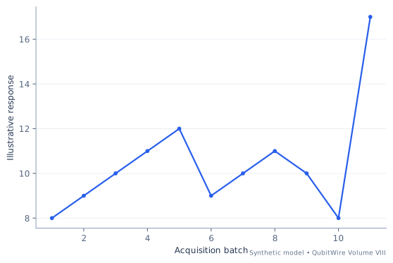
The constructed record compares an arithmetic mean, a median and a precisely defined trimmed mean. The extra disturbance is visible and synthetic, so its influence can be calculated exactly. The exercise does not argue that the median is universally superior. For an observable whose physical definition is an expectation value, replacing the mean with a different statistic can change the estimand rather than merely improve the estimate.
The explicitly supplied observations show how changing one point affects each summary. A real contamination model needs independent evidence. Documenting saturation, a known synchronization fault or a predetermined rejection rule is stronger than choosing whichever summary makes a desired conclusion look stable.
Start with the assumptions
- Eleven observations are explicitly constructed.
- The disturbance is added to one known record.
- No sampling distribution or confidence interval is inferred.
Mean = sum(x_i)/n
Median = the middle ordered observation for odd n
One-per-tail trimmed mean averages x_(2) through x_(n-1)
Compare the input regimes
Each case uses invented inputs. The results follow from this model and do not describe measured hardware.
Baseline regime
Complete inputs
- Ordinary noise scale
- 1
- Target level
- 10
- Single-batch disturbance
- 5
- Ordinary noise pattern
- -2, -1, 0, 1, 2, -1, 0, 1, 0, -2, 2
- Disturbed observation, one-based
- 11
- Observations trimmed from each tail
- 1
- The constructed eleven observations are 8, 9, 10, 11, 12, 9, 10, 11, 10, 8, 17. Only the final entry receives the declared extra disturbance.
- The arithmetic mean uses every magnitude and gives 10.454545. The median is the sixth sorted value, 10.
- Remove one observation from each sorted tail and average the remaining nine to obtain 10. This is a specified transformation, not permission to discard inconvenient measurements after seeing a result.
| Calculated quantity | Synthetic result |
|---|---|
| Arithmetic mean | 10.454545454545455 |
| Median | 10 |
| One-point-per-tail trimmed mean | 10 |
| Mean minus target | 0.45454545454545503 |
| Median minus target | 0 |
| Trimmed mean minus target | 0 |
| Batch | Response |
|---|---|
| 1 | 8 |
| 2 | 9 |
| 3 | 10 |
| 4 | 11 |
| 5 | 12 |
| 6 | 9 |
| 7 | 10 |
| 8 | 11 |
| 9 | 10 |
| 10 | 8 |
| 11 | 17 |
The disturbance shifts the mean by 0.454545 from the stipulated target. The comparison demonstrates influence, not a claim that a median estimates every physical observable correctly. For an expectation value defined as a mean, robust summaries can change the estimand and must be justified by a contamination model.
Comparison regime
Complete inputs
- Ordinary noise scale
- 1.5
- Target level
- 12.5
- Single-batch disturbance
- 20
- Ordinary noise pattern
- -2, -1, 0, 1, 2, -1, 0, 1, 0, -2, 2
- Disturbed observation, one-based
- 11
- Observations trimmed from each tail
- 1
- The constructed eleven observations are 9.5, 11, 12.5, 14, 15.5, 11, 12.5, 14, 12.5, 9.5, 35.5. Only the final entry receives the declared extra disturbance.
- The arithmetic mean uses every magnitude and gives 14.318182. The median is the sixth sorted value, 12.5.
- Remove one observation from each sorted tail and average the remaining nine to obtain 12.5. This is a specified transformation, not permission to discard inconvenient measurements after seeing a result.
| Calculated quantity | Synthetic result |
|---|---|
| Arithmetic mean | 14.318181818181818 |
| Median | 12.5 |
| One-point-per-tail trimmed mean | 12.5 |
| Mean minus target | 1.8181818181818183 |
| Median minus target | 0 |
| Trimmed mean minus target | 0 |
| Batch | Response |
|---|---|
| 1 | 9.5 |
| 2 | 11 |
| 3 | 12.5 |
| 4 | 14 |
| 5 | 15.5 |
| 6 | 11 |
| 7 | 12.5 |
| 8 | 14 |
| 9 | 12.5 |
| 10 | 9.5 |
| 11 | 35.5 |
The disturbance shifts the mean by 1.818182 from the stipulated target. The comparison demonstrates influence, not a claim that a median estimates every physical observable correctly. For an expectation value defined as a mean, robust summaries can change the estimand and must be justified by a contamination model.
Extended regime
Complete inputs
- Ordinary noise scale
- 2.1
- Target level
- 15.5
- Single-batch disturbance
- 38
- Ordinary noise pattern
- -2, -1, 0, 1, 2, -1, 0, 1, 0, -2, 2
- Disturbed observation, one-based
- 11
- Observations trimmed from each tail
- 1
- The constructed eleven observations are 11.3, 13.4, 15.5, 17.6, 19.7, 13.4, 15.5, 17.6, 15.5, 11.3, 57.7. Only the final entry receives the declared extra disturbance.
- The arithmetic mean uses every magnitude and gives 18.954545. The median is the sixth sorted value, 15.5.
- Remove one observation from each sorted tail and average the remaining nine to obtain 15.5. This is a specified transformation, not permission to discard inconvenient measurements after seeing a result.
| Calculated quantity | Synthetic result |
|---|---|
| Arithmetic mean | 18.954545454545453 |
| Median | 15.5 |
| One-point-per-tail trimmed mean | 15.5 |
| Mean minus target | 3.4545454545454533 |
| Median minus target | 0 |
| Trimmed mean minus target | 0 |
| Batch | Response |
|---|---|
| 1 | 11.3 |
| 2 | 13.4 |
| 3 | 15.5 |
| 4 | 17.6 |
| 5 | 19.7 |
| 6 | 13.4 |
| 7 | 15.5 |
| 8 | 17.6 |
| 9 | 15.5 |
| 10 | 11.3 |
| 11 | 57.7 |
The disturbance shifts the mean by 3.454545 from the stipulated target. The comparison demonstrates influence, not a claim that a median estimates every physical observable correctly. For an expectation value defined as a mean, robust summaries can change the estimand and must be justified by a contamination model.
Try the reasoning: If the physical quantity is an expectation value, what contamination model would justify replacing the arithmetic mean with a median?
Error control and measurement
Error control and measurementThe useful mitigation threshold is an error-budget crossoverHow many shots make a reduction in bias worth its extra variance?
An error-mitigated estimate can move closer to a reference on one run and farther away on another. That variation is expected when the procedure amplifies sampling noise. Judging the method by a single favorable estimate confuses chance with a repeatable improvement. A planning calculation needs a loss function that accounts for both the systematic offset and the spread.
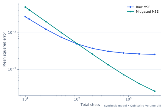
Mean squared error supplies a simple choice: variance plus squared bias. This lab stipulates a raw bias, a smaller residual bias after mitigation and a variance multiplier. With few shots, the added variance can dominate. With enough shots, a reduction in persistent bias can become more valuable. Equating the two expressions gives a transparent crossover rather than an unconditional claim that mitigation helps or hurts.
The assumed biases are the difficult inputs. They cannot normally be read directly from an unknown quantum answer. A trusted smaller problem, a controlled noise study or an independently justified model may provide evidence about them. The example therefore belongs beside a discussion of validation. It explains what would have to be known to choose a sample budget, while keeping the synthetic crossover separate from an experimentally established accuracy gain.
Start with the assumptions
- The multiplier gamma applies to variance, not standard deviation.
- Biases and shot variance are constant over the campaign.
- Both estimates target the same observable.
MSE_raw = b² + v/N
MSE_mitigated = b_m² + gamma v/N
N_cross = (gamma-1)v/(b²-b_m²), when the denominator is positive
Compare the input regimes
Each case uses invented inputs. The results follow from this model and do not describe measured hardware.
Baseline regime
Complete inputs
- Raw bias
- 0.05
- Residual mitigated bias
- 0.01
- Per-shot variance
- 0.25
- Variance multiplier
- 2
- Total shots
- 100
- Raw MSE = bias squared + sampling variance = 0.0025 + 0.0025.
- Mitigated MSE = residual bias squared + inflated sampling variance = 0.0001 + 0.005.
- Equating the MSEs gives N = 104.166667. Integer shot counts above that value favor mitigation in this model.
| Calculated quantity | Synthetic result |
|---|---|
| Raw mean squared error | 0.005000000000000001 |
| Mitigated mean squared error | 0.0051 |
| Raw root mean squared error | 0.07071067811865477 |
| Mitigated root mean squared error | 0.07141428428542851 |
| Continuous crossover shots | 104.16666666666664 |
At 100 shots, the raw estimate has lower modeled MSE. This is an accuracy comparison over repeated hypothetical experiments, not a judgment based on whichever single answer looks closer to an expected result. Biases must be independently characterized before using the model to plan an experiment.
Comparison regime
Complete inputs
- Raw bias
- 0.05
- Residual mitigated bias
- 0.02
- Per-shot variance
- 0.25
- Variance multiplier
- 2
- Total shots
- 3200
- Raw MSE = bias squared + sampling variance = 0.0025 + 7.8125e-05.
- Mitigated MSE = residual bias squared + inflated sampling variance = 0.0004 + 0.000156.
- Equating the MSEs gives N = 119.047619. Integer shot counts above that value favor mitigation in this model.
| Calculated quantity | Synthetic result |
|---|---|
| Raw mean squared error | 0.0025781250000000006 |
| Mitigated mean squared error | 0.00055625 |
| Raw root mean squared error | 0.05077524002897476 |
| Mitigated root mean squared error | 0.02358495283014151 |
| Continuous crossover shots | 119.04761904761904 |
At 3,200 shots, mitigation has lower modeled MSE. This is an accuracy comparison over repeated hypothetical experiments, not a judgment based on whichever single answer looks closer to an expected result. Biases must be independently characterized before using the model to plan an experiment.
Extended regime
Complete inputs
- Raw bias
- 0.05
- Residual mitigated bias
- 0.032
- Per-shot variance
- 0.25
- Variance multiplier
- 3
- Total shots
- 204800
- Raw MSE = bias squared + sampling variance = 0.0025 + 1.2207e-06.
- Mitigated MSE = residual bias squared + inflated sampling variance = 0.001024 + 3.66211e-06.
- Equating the MSEs gives N = 338.753388. Integer shot counts above that value favor mitigation in this model.
| Calculated quantity | Synthetic result |
|---|---|
| Raw mean squared error | 0.0025012207031250007 |
| Mitigated mean squared error | 0.0010276621093749999 |
| Raw root mean squared error | 0.05001220554149757 |
| Mitigated root mean squared error | 0.03205716939118299 |
| Continuous crossover shots | 338.75338753387524 |
At 204,800 shots, mitigation has lower modeled MSE. This is an accuracy comparison over repeated hypothetical experiments, not a judgment based on whichever single answer looks closer to an expected result. Biases must be independently characterized before using the model to plan an experiment.
Try the reasoning: At what shot budget does the lower modeled bias repay the extra variance? Explain why a single favorable estimate cannot establish that crossover.
Sources and model boundaries
- Error mitigation for short-depth quantum circuits ↗
Error-mitigation methods target expectation-value errors using techniques such as noise extrapolation and quasiprobability sampling. The MSE lab is an independently derived decision model; it does not attribute its assumed residual biases or variance multipliers to this paper.
Error control and measurementCalibrating more often can reduce the measurements you needHow should a refresh interval balance drifting bias against useful acquisition time?
Calibration consumes part of a campaign while attempting to make the remaining measurements more trustworthy. An extremely long interval spends almost all the time acquiring data, but measurements late in the interval may inherit a larger drift. An extremely short interval keeps data young while leaving little useful acquisition time. Neither extreme is automatically the best choice.
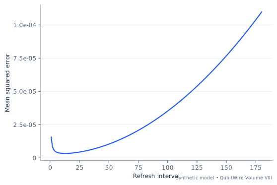
The model treats drift after a perfect calibration as a linear bias and assumes measurement ages are uniformly distributed across a repeated acquisition interval. Integrating the squared age-dependent bias gives a mean-squared drift contribution. A separate term reflects the smaller shot count caused by calibration downtime. Adding the two creates a concrete cadence problem whose optimum can be explored without claiming a real laboratory’s drift law is known.
The cases scan integer refresh intervals and compare the best tested choice with a declared reference schedule. They deliberately use a long-run duty-cycle approximation. A short campaign, imperfect calibration, interrupted schedules or random walk drift would need a different calculation. The useful article question is whether a reported improvement includes the time required to establish and maintain the operating point.
Start with the assumptions
- Each calibration resets bias exactly to zero.
- Bias then grows linearly at rate r.
- Campaign boundaries are neglected in the repeated-cycle approximation.
Useful fraction = L/(L+t_cal)
Expected shots = campaign_time × shot_rate × useful_fraction
MSE(L) = r² L²/3 + v/expected_shots
Compare the input regimes
Each case uses invented inputs. The results follow from this model and do not describe measured hardware.
Baseline regime
Complete inputs
- Campaign time
- 3600
- Calibration time
- 8
- Bias drift per time
- 0.0001
- Shots per useful time
- 40
- Per-shot variance
- 0.25
- Largest refresh interval
- 180
- Reference refresh interval
- 120
- An interval L leaves fraction L/(L + calibration time) for acquisition. At L = 13, that is 0.619048.
- Uniform age since a reset gives mean squared drift (r L)^2 / 3 = 5.63333e-07. Shot variance adds 2.80449e-06.
- Scan integer intervals 1 through 180; the best is 13. The reference interval 120 gives MSE 4.98519e-05.
| Calculated quantity | Synthetic result |
|---|---|
| Best tested refresh interval | 13 |
| Useful acquisition fraction | 0.6190476190476191 |
| Expected acquired shots | 89142.85714285714 |
| Best modeled MSE | 0.0000033678205128205124 |
| Reference-interval MSE | 0.000049851851851851855 |
| Reference / best MSE | 14.802407569547547 |
The best tested cadence is 13 time units. It is conditional on deterministic linear drift, a perfect reset and long-campaign duty-cycle accounting. If calibration leaves an offset or the drift is stochastic, both the age term and the optimum change. This model uses fractional expected shots; an actual schedule would need integer acquisitions and explicit start/end effects.
Comparison regime
Complete inputs
- Campaign time
- 3600
- Calibration time
- 18
- Bias drift per time
- 0.0006000000000000001
- Shots per useful time
- 90
- Per-shot variance
- 0.25
- Largest refresh interval
- 180
- Reference refresh interval
- 120
- An interval L leaves fraction L/(L + calibration time) for acquisition. At L = 4, that is 0.181818.
- Uniform age since a reset gives mean squared drift (r L)^2 / 3 = 1.92e-06. Shot variance adds 4.24383e-06.
- Scan integer intervals 1 through 180; the best is 4. The reference interval 120 gives MSE 0.001729.
| Calculated quantity | Synthetic result |
|---|---|
| Best tested refresh interval | 4 |
| Useful acquisition fraction | 0.18181818181818182 |
| Expected acquired shots | 58909.09090909091 |
| Best modeled MSE | 0.0000061638271604938274 |
| Reference-interval MSE | 0.0017288873456790127 |
| Reference / best MSE | 280.4892643259159 |
The best tested cadence is 4 time units. It is conditional on deterministic linear drift, a perfect reset and long-campaign duty-cycle accounting. If calibration leaves an offset or the drift is stochastic, both the age term and the optimum change. This model uses fractional expected shots; an actual schedule would need integer acquisitions and explicit start/end effects.
Extended regime
Complete inputs
- Campaign time
- 3600
- Calibration time
- 30
- Bias drift per time
- 0.0012000000000000001
- Shots per useful time
- 150
- Per-shot variance
- 0.25
- Largest refresh interval
- 180
- Reference refresh interval
- 120
- An interval L leaves fraction L/(L + calibration time) for acquisition. At L = 2, that is 0.0625.
- Uniform age since a reset gives mean squared drift (r L)^2 / 3 = 1.92e-06. Shot variance adds 7.40741e-06.
- Scan integer intervals 1 through 180; the best is 2. The reference interval 120 gives MSE 0.006913.
| Calculated quantity | Synthetic result |
|---|---|
| Best tested refresh interval | 2 |
| Useful acquisition fraction | 0.0625 |
| Expected acquired shots | 33750 |
| Best modeled MSE | 0.000009327407407407409 |
| Reference-interval MSE | 0.0069125787037037055 |
| Reference / best MSE | 741.1039747458705 |
The best tested cadence is 2 time units. It is conditional on deterministic linear drift, a perfect reset and long-campaign duty-cycle accounting. If calibration leaves an offset or the drift is stochastic, both the age term and the optimum change. This model uses fractional expected shots; an actual schedule would need integer acquisitions and explicit start/end effects.
Try the reasoning: If calibration no longer resets the bias exactly, which term would you add or replace before using the chosen refresh interval?
Error correction and systems
Error correction and systemsA code distance belongs to a workload, not a headlineHow much protection is needed when every logical operation exposes the machine for several rounds?
A small logical error probability is meaningful only beside the number of opportunities for failure. A memory experiment, a short logical operation and a large algorithm can tolerate very different per-round rates. Choosing a code distance therefore starts with a workload and an explicit accounting convention, rather than a desired number of decimal places.
The model assigns a simple distance-dependent logical error and makes each logical operation consume a number of correction rounds proportional to distance. Increasing distance improves one factor while increasing the exposure count, footprint and serial duration. The calculation then selects the smallest tested odd distance meeting a stated union-bound target. A union bound adds event probabilities and does not require the events to be independent, although the assumed per-location probabilities remain a strong physical modeling choice.
This is an accounting exercise, not a surface-code resource estimate for a named algorithm. A real implementation must also count factories, routing, boundaries, correlated faults, logical gate constructions and recovery behavior. Moving from per-location protection to complete-workload protection requires an explicit exposure count. The footprint must also state which resources it excludes.
Start with the assumptions
- The error law and coefficients are invented.
- A serial sequence of logical operations lasts d correction rounds per operation; all stored registers, including idle ones, remain exposed.
- All counted locations share the stipulated per-location bound.
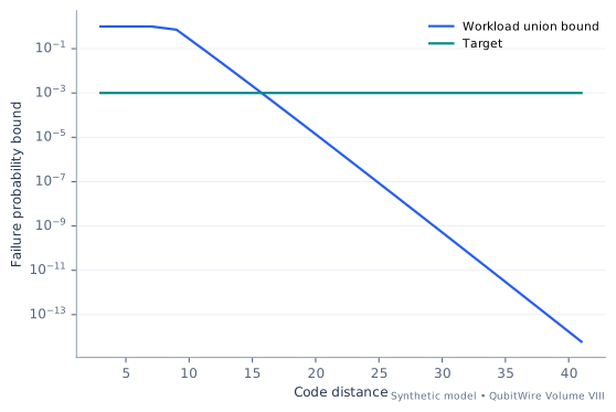
p_L(d) = A × ratio^((d+1)/2)
Counted locations = logical_registers × base_operations × d
Workload union bound = min(1, counted_locations × p_L)
Toy patch footprint = logical_registers × (2d²-1)
Compare the input regimes
Each case uses invented inputs. The results follow from this model and do not describe measured hardware.
Baseline regime
Complete inputs
- Physical error / model threshold
- 0.12
- Scaling prefactor
- 0.04
- Base logical operations
- 10000
- Logical registers
- 8
- Workload failure bound
- 0.001
- Cycle time, microseconds
- 1
- Tested odd distances
- 3, 5, 7, 9, 11, 13, 15, 17, 19, 21, 23, 25, 27, 29, 31, 33, 35, 37, 39, 41
- The error model gives p_L(d) = A × ratio^((d + 1)/2). Multiply by logical registers × base operations × distance to count the declared fault opportunities.
- At d = 17, the resulting union bound is min(1, 1,360,000 × 2.06391e-10) = 0.000281.
- The illustrative rotated-patch allocation is 8 × (2 × 17² - 1) = 4,616 physical qubits. The serial duration is 0.17 seconds. Routing space, factories and extra control patches are excluded.
| Calculated quantity | Synthetic result |
|---|---|
| Smallest passing tested distance | 17 |
| Chosen-distance logical error per location | 2.0639121407999993e-10 |
| Counted fault locations | 1360000 |
| Union-bound workload failure | 0.0002806920511487999 |
| Illustrative physical-qubit footprint | 4616 |
| Serial operation time, seconds | 0.17 |
| Distance | Per-location error | Counted locations | Workload failure bound | Physical qubits | Seconds |
|---|---|---|---|---|---|
| 3 | 0.000576 | 240000 | 1 | 136 | 0.03 |
| 5 | 0.00006911999999999999 | 400000 | 1 | 392 | 0.05 |
| 7 | 0.000008294399999999998 | 560000 | 1 | 776 | 0.07 |
| 9 | 9.95328e-7 | 720000 | 0.71663616 | 1288 | 0.09 |
| 11 | 1.1943935999999997e-7 | 880000 | 0.10510663679999997 | 1928 | 0.11 |
| 13 | 1.4332723199999996e-8 | 1040000 | 0.014906032127999996 | 2696 | 0.13 |
| 15 | 1.7199267839999996e-9 | 1200000 | 0.0020639121407999995 | 3592 | 0.15 |
| 17 | 2.0639121407999993e-10 | 1360000 | 0.0002806920511487999 | 4616 | 0.17 |
| 19 | 2.476694568959999e-11 | 1520000 | 0.00003764575744819199 | 5768 | 0.19 |
| 21 | 2.9720334827519992e-12 | 1680000 | 0.000004993016251023359 | 7048 | 0.21 |
| 23 | 3.5664401793023986e-13 | 1840000 | 6.562249929916414e-7 | 8456 | 0.23 |
| 25 | 4.2797282151628786e-14 | 2000000 | 8.559456430325757e-8 | 9992 | 0.25 |
| 27 | 5.135673858195453e-15 | 2160000 | 1.1093055533702179e-8 | 11656 | 0.27 |
| 29 | 6.162808629834545e-16 | 2320000 | 1.4297716021216143e-9 | 13448 | 0.29 |
| 31 | 7.395370355801452e-17 | 2480000 | 1.8340518482387603e-10 | 15368 | 0.31 |
| 33 | 8.874444426961742e-18 | 2640000 | 2.3428533287178998e-11 | 17416 | 0.33 |
| 35 | 1.064933331235409e-18 | 2800000 | 2.981813327459145e-12 | 19592 | 0.35 |
| 37 | 1.277919997482491e-19 | 2960000 | 3.7826431925481733e-13 | 21896 | 0.37 |
| 39 | 1.533503996978989e-20 | 3120000 | 4.784532470574446e-14 | 24328 | 0.39 |
| 41 | 1.8402047963747867e-21 | 3280000 | 6.0358717321093e-15 | 26888 | 0.41 |
Distance 17 is the smallest tested odd distance meeting the stated target. The gate count alone is not the exposure count: this model makes each logical operation last d rounds. Its scaling prefactor and threshold ratio are invented. No threshold theorem or device forecast is inferred from the scan.
Comparison regime
Complete inputs
- Physical error / model threshold
- 0.245
- Scaling prefactor
- 0.04
- Base logical operations
- 60000
- Logical registers
- 18
- Workload failure bound
- 0.001
- Cycle time, microseconds
- 1.5
- Tested odd distances
- 3, 5, 7, 9, 11, 13, 15, 17, 19, 21, 23, 25, 27, 29, 31, 33, 35, 37, 39, 41
- The error model gives p_L(d) = A × ratio^((d + 1)/2). Multiply by logical registers × base operations × distance to count the declared fault opportunities.
- At d = 29, the resulting union bound is min(1, 31,320,000 × 2.75138e-11) = 0.000862.
- The illustrative rotated-patch allocation is 18 × (2 × 29² - 1) = 30,258 physical qubits. The serial duration is 2.61 seconds. Routing space, factories and extra control patches are excluded.
| Calculated quantity | Synthetic result |
|---|---|
| Smallest passing tested distance | 29 |
| Chosen-distance logical error per location | 2.7513843128286442e-11 |
| Counted fault locations | 31320000 |
| Union-bound workload failure | 0.0008617335667779314 |
| Illustrative physical-qubit footprint | 30258 |
| Serial operation time, seconds | 2.61 |
| Distance | Per-location error | Counted locations | Workload failure bound | Physical qubits | Seconds |
|---|---|---|---|---|---|
| 3 | 0.002401 | 3240000 | 1 | 306 | 0.27 |
| 5 | 0.0005882449999999999 | 5400000 | 1 | 882 | 0.45 |
| 7 | 0.00014412002499999998 | 7560000 | 1 | 1746 | 0.63 |
| 9 | 0.000035309406125 | 9720000 | 1 | 2898 | 0.81 |
| 11 | 0.000008650804500625 | 11880000 | 1 | 4338 | 0.99 |
| 13 | 0.000002119447102653125 | 14040000 | 1 | 6066 | 1.17 |
| 15 | 5.192645401500155e-7 | 16200000 | 1 | 8082 | 1.35 |
| 17 | 1.272198123367538e-7 | 18360000 | 1 | 10386 | 1.53 |
| 19 | 3.116885402250468e-8 | 20520000 | 0.639584884541796 | 12978 | 1.71 |
| 21 | 7.636369235513648e-9 | 22680000 | 0.17319285426144954 | 15858 | 1.89 |
| 23 | 1.8709104627008436e-9 | 24840000 | 0.046473415893488954 | 19026 | 2.07 |
| 25 | 4.5837306336170665e-10 | 27000000 | 0.01237607271076608 | 22482 | 2.25 |
| 27 | 1.1230140052361812e-10 | 29160000 | 0.0032747088392687043 | 26226 | 2.43 |
| 29 | 2.7513843128286442e-11 | 31320000 | 0.0008617335667779314 | 30258 | 2.61 |
| 31 | 6.740891566430178e-12 | 33480000 | 0.00022568504964408235 | 34578 | 2.79 |
| 33 | 1.6515184337753934e-12 | 35640000 | 0.00005886011697975502 | 39186 | 2.97 |
| 35 | 4.046220162749714e-13 | 37800000 | 0.000015294712215193918 | 44082 | 3.15 |
| 37 | 9.913239398736799e-14 | 39960000 | 0.000003961330463735225 | 49266 | 3.33 |
| 39 | 2.428743652690516e-14 | 42120000 | 0.0000010229868265132453 | 54738 | 3.51 |
| 41 | 5.950421949091763e-15 | 44280000 | 2.634846839057833e-7 | 60498 | 3.69 |
Distance 29 is the smallest tested odd distance meeting the stated target. The gate count alone is not the exposure count: this model makes each logical operation last d rounds. Its scaling prefactor and threshold ratio are invented. No threshold theorem or device forecast is inferred from the scan.
Extended regime
Complete inputs
- Physical error / model threshold
- 0.395
- Scaling prefactor
- 0.04
- Base logical operations
- 120000
- Logical registers
- 30
- Workload failure bound
- 0.001
- Cycle time, microseconds
- 2.1
- Tested odd distances
- 3, 5, 7, 9, 11, 13, 15, 17, 19, 21, 23, 25, 27, 29, 31, 33, 35, 37, 39, 41
- The error model gives p_L(d) = A × ratio^((d + 1)/2). Multiply by logical registers × base operations × distance to count the declared fault opportunities.
- At d = 41, the resulting union bound is min(1, 147,600,000 × 1.35082e-10) = 0.019938.
- The illustrative rotated-patch allocation is 30 × (2 × 41² - 1) = 100,830 physical qubits. The serial duration is 10.332 seconds. Routing space, factories and extra control patches are excluded.
| Calculated quantity | Synthetic result |
|---|---|
| Smallest passing tested distance | No tested distance passes |
| Chosen-distance logical error per location | 1.3508247196523e-10 |
| Counted fault locations | 147600000 |
| Union-bound workload failure | 0.01993817286206795 |
| Illustrative physical-qubit footprint | 100830 |
| Serial operation time, seconds | 10.332 |
| Distance | Per-location error | Counted locations | Workload failure bound | Physical qubits | Seconds |
|---|---|---|---|---|---|
| 3 | 0.006241000000000001 | 10800000 | 1 | 510 | 0.756 |
| 5 | 0.0024651950000000003 | 18000000 | 1 | 1470 | 1.26 |
| 7 | 0.0009737520250000003 | 25200000 | 1 | 2910 | 1.764 |
| 9 | 0.00038463204987500006 | 32400000 | 1 | 4830 | 2.268 |
| 11 | 0.00015192965970062505 | 39600000 | 1 | 7230 | 2.772 |
| 13 | 0.0000600122155817469 | 46800000 | 1 | 10110 | 3.276 |
| 15 | 0.000023704825154790025 | 54000000 | 1 | 13470 | 3.78 |
| 17 | 0.00000936340593614206 | 61200000 | 1 | 17310 | 4.284 |
| 19 | 0.000003698545344776114 | 68400000 | 1 | 21630 | 4.788 |
| 21 | 0.0000014609254111865652 | 75600000 | 1 | 26430 | 5.292 |
| 23 | 5.770655374186932e-7 | 82800000 | 1 | 31710 | 5.796 |
| 25 | 2.2794088728038384e-7 | 90000000 | 1 | 37470 | 6.3 |
| 27 | 9.003665047575162e-8 | 97200000 | 1 | 43710 | 6.804 |
| 29 | 3.556447693792189e-8 | 104400000 | 1 | 50430 | 7.308 |
| 31 | 1.4047968390479147e-8 | 111600000 | 1 | 57630 | 7.812 |
| 33 | 5.548947514239264e-9 | 118800000 | 0.6592149646916245 | 65310 | 8.316 |
| 35 | 2.191834268124509e-9 | 126000000 | 0.27617111778368814 | 73470 | 8.82 |
| 37 | 8.657745359091812e-10 | 133200000 | 0.11532116818310294 | 82110 | 9.324 |
| 39 | 3.419809416841266e-10 | 140400000 | 0.048014124212451374 | 91230 | 9.828 |
| 41 | 1.3508247196523e-10 | 147600000 | 0.01993817286206795 | 100830 | 10.332 |
The tested distance range does not meet the target. The gate count alone is not the exposure count: this model makes each logical operation last d rounds. Its scaling prefactor and threshold ratio are invented. No threshold theorem or device forecast is inferred from the scan.
Try the reasoning: Double the number of stored logical registers. Which costs and failure opportunities increase even if the serial operation count stays fixed?
Sources and model boundaries
- Surface codes: Towards practical large-scale quantum computation ↗
Surface-code computation requires physical layouts, repeated stabilizer information and logical operation constructions with resource costs. Only architectural context is used. All scaling coefficients and workload values in the lab are invented, and the toy footprint excludes substantial resources.
Error correction and systemsA quiet average can hide a decoder’s busiest minuteWill the decoder respond in time when slow jobs arrive in bursts?
A decoder is a classical computation attached to a quantum experiment. Its response can become part of a time-critical feedback path. Average throughput describes whether work is usually sustainable, while individual response times reveal what happens to the jobs that encounter a backlog. Both are needed to interpret a claim about operating speed.
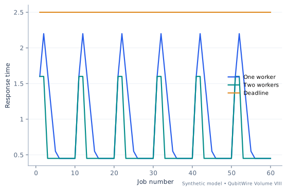
This laboratory uses a deterministic arrival trace and makes the first two service times in each block longer. A single worker can have an average service time below the arrival spacing and still miss deadlines after those bursts. A second worker changes the schedule, but it does not make either individual service operation faster. The distinction separates hardware acceleration from queue management.
The exact trace is supplied with each worked case, making the result reproducible without a random seed. It is intentionally a classical queue simulation. Real decoders can have batch dependencies, shared memory, communication bottlenecks and different requirements for when an answer becomes necessary. The Model page can use this trace to explain what a latency histogram adds to a mean-speed number, while leaving quantum error-correction performance to its own evidence.
Start with the assumptions
- Jobs can use any available identical worker.
- There are no inter-job dependencies or transfer costs.
- The burst pattern and service times are stipulated.
start_i = max(arrival_i, earliest worker-free time)
finish_i = start_i + service_i
response_i = finish_i - arrival_i; miss if response_i > deadline
Compare the input regimes
Each case uses invented inputs. The results follow from this model and do not describe measured hardware.
Baseline regime
Complete inputs
- Arrival spacing
- 1
- Normal service time
- 0.45
- Burst service time
- 1.6
- Burst period
- 10
- Response deadline
- 2.5
- Jobs in trace
- 60
- Burst jobs at start of each period
- 2
- Create 60 arrivals separated by 1 time units. The first two jobs in every 10-job block use burst service 1.6.
- For each arrival, select the first available worker; start at max(arrival time, worker-free time). Completion minus arrival is the response time.
- The one-worker queue misses 0 deadlines. The two-worker schedule misses 0 under exactly the same arrival and service trace.
| Calculated quantity | Synthetic result |
|---|---|
| Mean service / arrival spacing | 0.68 |
| One-worker maximum response time | 2.200000000000003 |
| One-worker missed deadlines | 0 |
| Two-worker maximum response time | 1.6000000000000014 |
| Two-worker missed deadlines | 0 |
| One-worker maximum wait before service | 1.2000000000000028 |
| Job | Service time | One-worker response | Two-worker response |
|---|---|---|---|
| 1 | 1.6 | 1.6 | 1.6 |
| 2 | 1.6 | 2.2 | 1.6 |
| 3 | 0.45 | 1.6500000000000004 | 0.4500000000000002 |
| 4 | 0.45 | 1.1000000000000005 | 0.4500000000000002 |
| 5 | 0.45 | 0.5500000000000007 | 0.4500000000000002 |
| 6 | 0.45 | 0.4500000000000002 | 0.4500000000000002 |
| 7 | 0.45 | 0.4500000000000002 | 0.4500000000000002 |
| 8 | 0.45 | 0.4500000000000002 | 0.4500000000000002 |
| 9 | 0.45 | 0.4499999999999993 | 0.4499999999999993 |
| 10 | 0.45 | 0.4499999999999993 | 0.4499999999999993 |
| 11 | 1.6 | 1.5999999999999996 | 1.5999999999999996 |
| 12 | 1.6 | 2.1999999999999993 | 1.5999999999999996 |
The average utilization proxy is 0.68, while the maximum one-worker response is 2.2. A mean below one does not rule out burst-related deadline failures. The second worker is a scheduling experiment; real decoding may have dependencies, memory contention and communication costs omitted here.
Comparison regime
Complete inputs
- Arrival spacing
- 1
- Normal service time
- 0.575
- Burst service time
- 2.5
- Burst period
- 12
- Response deadline
- 2.6
- Jobs in trace
- 60
- Burst jobs at start of each period
- 2
- Create 60 arrivals separated by 1 time units. The first two jobs in every 12-job block use burst service 2.5.
- For each arrival, select the first available worker; start at max(arrival time, worker-free time). Completion minus arrival is the response time.
- The one-worker queue misses 20 deadlines. The two-worker schedule misses 0 under exactly the same arrival and service trace.
| Calculated quantity | Synthetic result |
|---|---|
| Mean service / arrival spacing | 0.8958333333333333 |
| One-worker maximum response time | 4 |
| One-worker missed deadlines | 20 |
| Two-worker maximum response time | 2.5 |
| Two-worker missed deadlines | 0 |
| One-worker maximum wait before service | 3 |
| Job | Service time | One-worker response | Two-worker response |
|---|---|---|---|
| 1 | 2.5 | 2.5 | 2.5 |
| 2 | 2.5 | 4 | 2.5 |
| 3 | 0.575 | 3.575 | 1.0750000000000002 |
| 4 | 0.575 | 3.1500000000000004 | 0.6500000000000004 |
| 5 | 0.575 | 2.7250000000000005 | 0.5750000000000002 |
| 6 | 0.575 | 2.3000000000000007 | 0.5750000000000002 |
| 7 | 0.575 | 1.8750000000000009 | 0.5750000000000002 |
| 8 | 0.575 | 1.450000000000001 | 0.5750000000000002 |
| 9 | 0.575 | 1.0250000000000004 | 0.5749999999999993 |
| 10 | 0.575 | 0.5999999999999996 | 0.5749999999999993 |
| 11 | 0.575 | 0.5749999999999993 | 0.5749999999999993 |
| 12 | 0.575 | 0.5749999999999993 | 0.5749999999999993 |
The average utilization proxy is 0.895833, while the maximum one-worker response is 4. A mean below one does not rule out burst-related deadline failures. The second worker is a scheduling experiment; real decoding may have dependencies, memory contention and communication costs omitted here.
Extended regime
Complete inputs
- Arrival spacing
- 1
- Normal service time
- 0.7250000000000001
- Burst service time
- 3.58
- Burst period
- 12
- Response deadline
- 2.8
- Jobs in trace
- 60
- Burst jobs at start of each period
- 2
- Create 60 arrivals separated by 1 time units. The first two jobs in every 12-job block use burst service 3.58.
- For each arrival, select the first available worker; start at max(arrival time, worker-free time). Completion minus arrival is the response time.
- The one-worker queue misses 60 deadlines. The two-worker schedule misses 10 under exactly the same arrival and service trace.
| Calculated quantity | Synthetic result |
|---|---|
| Mean service / arrival spacing | 1.2008333333333334 |
| One-worker maximum response time | 15.800000000000026 |
| One-worker missed deadlines | 60 |
| Two-worker maximum response time | 3.58 |
| Two-worker missed deadlines | 10 |
| One-worker maximum wait before service | 14.800000000000026 |
| Job | Service time | One-worker response | Two-worker response |
|---|---|---|---|
| 1 | 3.58 | 3.58 | 3.58 |
| 2 | 3.58 | 6.16 | 3.58 |
| 3 | 0.7250000000000001 | 5.885 | 2.3049999999999997 |
| 4 | 0.7250000000000001 | 5.609999999999999 | 2.0299999999999994 |
| 5 | 0.7250000000000001 | 5.334999999999999 | 1.3049999999999997 |
| 6 | 0.7250000000000001 | 5.059999999999999 | 0.754999999999999 |
| 7 | 0.7250000000000001 | 4.784999999999998 | 0.7249999999999996 |
| 8 | 0.7250000000000001 | 4.509999999999998 | 0.7249999999999996 |
| 9 | 0.7250000000000001 | 4.234999999999998 | 0.7249999999999996 |
| 10 | 0.7250000000000001 | 3.9599999999999973 | 0.7249999999999996 |
| 11 | 0.7250000000000001 | 3.684999999999997 | 0.7249999999999996 |
| 12 | 0.7250000000000001 | 3.4099999999999966 | 0.7249999999999996 |
The average utilization proxy is 1.200833, while the maximum one-worker response is 15.8. A mean below one does not rule out burst-related deadline failures. The second worker is a scheduling experiment; real decoding may have dependencies, memory contention and communication costs omitted here.
Try the reasoning: Find a regime with a mean service time below the arrival spacing but a missed deadline. Which burst causes it?
Error correction and systemsEnough resources across the day may still be too lateHow large a reserve keeps a bursty computation supplied?
A quantum computation may need a special resource in bursts while its production machinery works at a steadier pace. Total production can exceed total demand and still fail to serve the schedule, because the resource arrives after the moment it was needed. A supply-rate number by itself cannot settle that timing question.
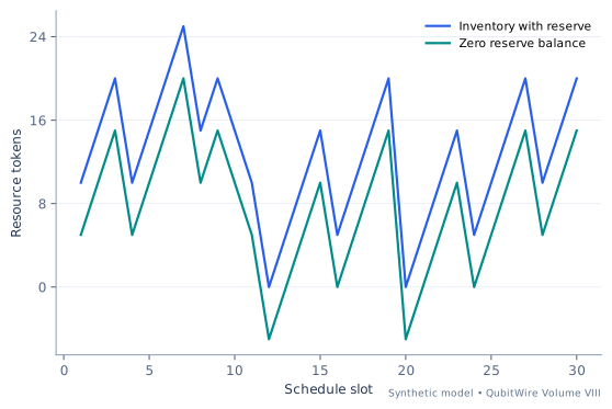
The constructed schedule treats production and demand as tokens at discrete boundaries. Three slots have no production, and repeated demand bursts create deficits. The smallest initial reserve is determined by the deepest cumulative deficit. After adding that reserve, the highest resulting inventory gives a boundary-capacity requirement. This makes two design questions visible: how much stock must exist before the computation starts, and how much can accumulate later.
If the tokens represent quantum states, the classical balance is only a first layer. States may age, occupy protected qubits, fail a quality test or be consumed by failed operations. The example therefore belongs beside a resource factory explanation with its scope stated clearly. It offers an exact demand-planning calculation without implying that quantum states are interchangeable durable objects in a warehouse.
Start with the assumptions
- Supply and demand are netted simultaneously at each boundary.
- Stored tokens neither expire nor lose quality in this calculation.
- All requested tokens have the same resource meaning.
Cumulative net supply at slot t = sum_{i<=t}(supply_i-demand_i)
Minimum initial reserve = max(0, -minimum cumulative net supply)
Boundary capacity = maximum(initial reserve + cumulative net supply), including time zero
Compare the input regimes
Each case uses invented inputs. The results follow from this model and do not describe measured hardware.
Baseline regime
Complete inputs
- Supply per slot
- 10
- Base demand per slot
- 5
- Burst demand
- 15
- Burst period
- 4
- Schedule slots
- 30
- Zero-supply slots, one-based
- 10, 11, 20
- Supply is zero in slots 10, 11 and 20; all other slots produce 10 tokens. Demand includes the declared periodic bursts.
- Cumulative net production reaches a minimum of -5. An initial reserve of max(0, -minimum) = 5 prevents a negative end-of-slot balance.
- Add that reserve to every cumulative value. The largest start/end boundary inventory is 25; final stock is 20. Supply and demand are netted simultaneously at each boundary.
| Calculated quantity | Synthetic result |
|---|---|
| Total produced tokens | 270 |
| Total requested tokens | 255 |
| Minimum initial reserve | 5 |
| Required capacity at slot boundaries | 25 |
| Final inventory with that reserve | 20 |
| Supply-minus-demand over campaign | 15 |
| Slot | Supply | Demand | Inventory with reserve |
|---|---|---|---|
| 1 | 10 | 5 | 10 |
| 2 | 10 | 5 | 15 |
| 3 | 10 | 5 | 20 |
| 4 | 10 | 20 | 10 |
| 5 | 10 | 5 | 15 |
| 6 | 10 | 5 | 20 |
| 7 | 10 | 5 | 25 |
| 8 | 10 | 20 | 15 |
| 9 | 10 | 5 | 20 |
| 10 | 0 | 5 | 15 |
| 11 | 0 | 5 | 10 |
| 12 | 10 | 20 | 0 |
| 13 | 10 | 5 | 5 |
| 14 | 10 | 5 | 10 |
| 15 | 10 | 5 | 15 |
| 16 | 10 | 20 | 5 |
| 17 | 10 | 5 | 10 |
| 18 | 10 | 5 | 15 |
| 19 | 10 | 5 | 20 |
| 20 | 0 | 20 | 0 |
| 21 | 10 | 5 | 5 |
| 22 | 10 | 5 | 10 |
| 23 | 10 | 5 | 15 |
| 24 | 10 | 20 | 5 |
| 25 | 10 | 5 | 10 |
| 26 | 10 | 5 | 15 |
| 27 | 10 | 5 | 20 |
| 28 | 10 | 20 | 10 |
| 29 | 10 | 5 | 15 |
| 30 | 10 | 5 | 20 |
The toy schedule needs 5 stored tokens before it begins, even though net production across the campaign is 15. A reserve addresses timing, not state quality. If tokens represent prepared quantum resources, finite storage lifetime and extra storage qubits require a separate physical model.
Comparison regime
Complete inputs
- Supply per slot
- 11
- Base demand per slot
- 7
- Burst demand
- 30
- Burst period
- 6
- Schedule slots
- 30
- Zero-supply slots, one-based
- 10, 11, 20
- Supply is zero in slots 10, 11 and 20; all other slots produce 11 tokens. Demand includes the declared periodic bursts.
- Cumulative net production reaches a minimum of -63. An initial reserve of max(0, -minimum) = 63 prevents a negative end-of-slot balance.
- Add that reserve to every cumulative value. The largest start/end boundary inventory is 83; final stock is 0. Supply and demand are netted simultaneously at each boundary.
| Calculated quantity | Synthetic result |
|---|---|
| Total produced tokens | 297 |
| Total requested tokens | 360 |
| Minimum initial reserve | 63 |
| Required capacity at slot boundaries | 83 |
| Final inventory with that reserve | 0 |
| Supply-minus-demand over campaign | -63 |
| Slot | Supply | Demand | Inventory with reserve |
|---|---|---|---|
| 1 | 11 | 7 | 67 |
| 2 | 11 | 7 | 71 |
| 3 | 11 | 7 | 75 |
| 4 | 11 | 7 | 79 |
| 5 | 11 | 7 | 83 |
| 6 | 11 | 37 | 57 |
| 7 | 11 | 7 | 61 |
| 8 | 11 | 7 | 65 |
| 9 | 11 | 7 | 69 |
| 10 | 0 | 7 | 62 |
| 11 | 0 | 7 | 55 |
| 12 | 11 | 37 | 29 |
| 13 | 11 | 7 | 33 |
| 14 | 11 | 7 | 37 |
| 15 | 11 | 7 | 41 |
| 16 | 11 | 7 | 45 |
| 17 | 11 | 7 | 49 |
| 18 | 11 | 37 | 23 |
| 19 | 11 | 7 | 27 |
| 20 | 0 | 7 | 20 |
| 21 | 11 | 7 | 24 |
| 22 | 11 | 7 | 28 |
| 23 | 11 | 7 | 32 |
| 24 | 11 | 37 | 6 |
| 25 | 11 | 7 | 10 |
| 26 | 11 | 7 | 14 |
| 27 | 11 | 7 | 18 |
| 28 | 11 | 7 | 22 |
| 29 | 11 | 7 | 26 |
| 30 | 11 | 37 | 0 |
The toy schedule needs 63 stored tokens before it begins, even though net production across the campaign is -63. A reserve addresses timing, not state quality. If tokens represent prepared quantum resources, finite storage lifetime and extra storage qubits require a separate physical model.
Extended regime
Complete inputs
- Supply per slot
- 13
- Base demand per slot
- 7
- Burst demand
- 48
- Burst period
- 6
- Schedule slots
- 30
- Zero-supply slots, one-based
- 10, 11, 20
- Supply is zero in slots 10, 11 and 20; all other slots produce 13 tokens. Demand includes the declared periodic bursts.
- Cumulative net production reaches a minimum of -99. An initial reserve of max(0, -minimum) = 99 prevents a negative end-of-slot balance.
- Add that reserve to every cumulative value. The largest start/end boundary inventory is 129; final stock is 0. Supply and demand are netted simultaneously at each boundary.
| Calculated quantity | Synthetic result |
|---|---|
| Total produced tokens | 351 |
| Total requested tokens | 450 |
| Minimum initial reserve | 99 |
| Required capacity at slot boundaries | 129 |
| Final inventory with that reserve | 0 |
| Supply-minus-demand over campaign | -99 |
| Slot | Supply | Demand | Inventory with reserve |
|---|---|---|---|
| 1 | 13 | 7 | 105 |
| 2 | 13 | 7 | 111 |
| 3 | 13 | 7 | 117 |
| 4 | 13 | 7 | 123 |
| 5 | 13 | 7 | 129 |
| 6 | 13 | 55 | 87 |
| 7 | 13 | 7 | 93 |
| 8 | 13 | 7 | 99 |
| 9 | 13 | 7 | 105 |
| 10 | 0 | 7 | 98 |
| 11 | 0 | 7 | 91 |
| 12 | 13 | 55 | 49 |
| 13 | 13 | 7 | 55 |
| 14 | 13 | 7 | 61 |
| 15 | 13 | 7 | 67 |
| 16 | 13 | 7 | 73 |
| 17 | 13 | 7 | 79 |
| 18 | 13 | 55 | 37 |
| 19 | 13 | 7 | 43 |
| 20 | 0 | 7 | 36 |
| 21 | 13 | 7 | 42 |
| 22 | 13 | 7 | 48 |
| 23 | 13 | 7 | 54 |
| 24 | 13 | 55 | 12 |
| 25 | 13 | 7 | 18 |
| 26 | 13 | 7 | 24 |
| 27 | 13 | 7 | 30 |
| 28 | 13 | 7 | 36 |
| 29 | 13 | 7 | 42 |
| 30 | 13 | 55 | 0 |
The toy schedule needs 99 stored tokens before it begins, even though net production across the campaign is -99. A reserve addresses timing, not state quality. If tokens represent prepared quantum resources, finite storage lifetime and extra storage qubits require a separate physical model.
Try the reasoning: Would the same reserve suffice if each slot demanded its tokens before new supply arrived? State the within-slot ordering explicitly.
Error correction and systemsSpare modules cannot repair a shared failureWhere does a redundancy calculation stop improving availability?
A modular system can tolerate some components being unavailable if enough working modules remain to perform the task. That is a capacity requirement, which differs from demanding that every installed component work simultaneously. Adding spares can increase the chance of meeting it under a model of independent failures.
Independence is also the assumption most likely to make a reliability calculation look too optimistic. Modules may share power, timing, network equipment, software updates or operating staff. A common outage can remove the entire service even when each module’s individual availability appears excellent. This lab adds one explicit common event to a binomial module model so the effect can be calculated rather than buried in a footnote.
The resulting ceiling is easy to interpret: no number of otherwise independent spares can exceed the probability that the shared service is available. The cases do not estimate a real vendor’s uptime. They create a disciplined question for a directory or infrastructure article: which failures are independent enough for redundancy to help, and which require diversity or a redesigned shared dependency?
Start with the assumptions
- The common outage removes all capacity.
- Outside that event, module availability is independent and identical.
- Exactly k active modules suffice for the declared workload.
P(enough active modules) = sum_{j=k}^n C(n,j)a^j(1-a)^(n-j)
Usable probability with shared outage q = (1-q) × P(enough active)
Common-mode ceiling = 1-q
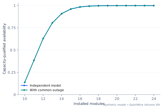
Compare the input regimes
Each case uses invented inputs. The results follow from this model and do not describe measured hardware.
Baseline regime
Complete inputs
- Installed modules
- 12
- Required active modules
- 10
- Independent module availability
- 0.82
- Common outage probability
- 0.002
- With no common outage, sum the binomial probabilities for 10 through 12 active modules.
- The independent capacity probability is 0.629787. Multiply by 0.998, the chance the shared service is available.
- Even infinitely many otherwise adequate independent modules cannot exceed the common-mode ceiling 0.998 in this model.
| Calculated quantity | Synthetic result |
|---|---|
| Capacity-qualified independent availability | 0.6297868795813713 |
| Availability including common outage | 0.6285273058222085 |
| Common-mode ceiling | 0.998 |
| Expected active modules without common outage | 9.84 |
| Expected active modules including common outage | 9.820319999999999 |
The installed system has modeled usable capacity probability 0.628527. Extra modules protect against independent outages while the shared failure mode persists. The common outage is an explicit invented mechanism; the independence calculation must not be used as a measured reliability claim for a real modular quantum machine.
Comparison regime
Complete inputs
- Installed modules
- 17
- Required active modules
- 11
- Independent module availability
- 0.8799999999999999
- Common outage probability
- 0.017
- With no common outage, sum the binomial probabilities for 11 through 17 active modules.
- The independent capacity probability is 0.997678. Multiply by 0.983, the chance the shared service is available.
- Even infinitely many otherwise adequate independent modules cannot exceed the common-mode ceiling 0.983 in this model.
| Calculated quantity | Synthetic result |
|---|---|
| Capacity-qualified independent availability | 0.9976779468023482 |
| Availability including common outage | 0.9807174217067083 |
| Common-mode ceiling | 0.983 |
| Expected active modules without common outage | 14.959999999999997 |
| Expected active modules including common outage | 14.705679999999997 |
The installed system has modeled usable capacity probability 0.980717. Extra modules protect against independent outages while the shared failure mode persists. The common outage is an explicit invented mechanism; the independence calculation must not be used as a measured reliability claim for a real modular quantum machine.
Extended regime
Complete inputs
- Installed modules
- 23
- Required active modules
- 13
- Independent module availability
- 0.952
- Common outage probability
- 0.035
- With no common outage, sum the binomial probabilities for 13 through 23 active modules.
- The independent capacity probability is 1. Multiply by 0.965, the chance the shared service is available.
- Even infinitely many otherwise adequate independent modules cannot exceed the common-mode ceiling 0.965 in this model.
| Calculated quantity | Synthetic result |
|---|---|
| Capacity-qualified independent availability | 0.9999999975419924 |
| Availability including common outage | 0.9649999976280227 |
| Common-mode ceiling | 0.965 |
| Expected active modules without common outage | 21.896 |
| Expected active modules including common outage | 21.12964 |
The installed system has modeled usable capacity probability 0.965. Extra modules protect against independent outages while the shared failure mode persists. The common outage is an explicit invented mechanism; the independence calculation must not be used as a measured reliability claim for a real modular quantum machine.
Try the reasoning: Can adding independent modules overcome the common outage ceiling? Which component would need a different reliability model?
Quantum networking
Quantum networkingA finite memory changes whether two quantum links meetHow much does a short storage window improve completion before a deadline?
Two probabilistic links rarely succeed on the same attempt when each has a small heralding probability. Memory can preserve the first success while the second link keeps trying. But an unlimited-memory formula can hide the central engineering constraint: a state may cease to be useful before its partner arrives.
The discrete model tracks whether the request is empty, holds an A herald or holds a B herald, and how many partner-attempt slots remain before expiry. Completion is absorbing. Every time step transfers probability among these states, so the complete deadline probability can be calculated without sampling noise. The accompanying trace checks that completed and unfinished probability still sum to one.
A hard cutoff is deliberately simpler than physical decoherence. The stored state is granted full eligibility until its final valid slot and none afterward. This lets the reader isolate timing and compare no memory, a finite window and memory that lasts to the deadline. A physical networking article would additionally need storage efficiencies, state-quality measurements, swapping success, classical latency and a task-specific definition of usefulness.
Start with the assumptions
- Link attempts are independent with stationary probabilities.
- Only the missing link is attempted while one herald is held.
- A stored herald remains valid for the declared number of additional slots.
Empty-state simultaneous completion probability per slot = p_A p_B
A-held completion probability per partner attempt = p_B
Deadline probability follows exact finite-state probability propagation
Expected capped completion time = sum_{t=0}^{H-1} P(not complete after t slots)
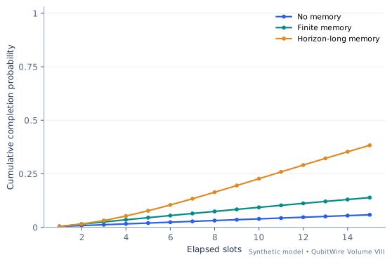
Compare the input regimes
Each case uses invented inputs. The results follow from this model and do not describe measured hardware.
Baseline regime
Complete inputs
- Link A success per slot
- 0.08
- Link B success per slot
- 0.05
- Additional slots a stored herald remains valid
- 1
- Deadline slots
- 15
- Start empty. Each slot gives independent probabilities 0.08 and 0.05 for the two links. Simultaneous success ends the request.
- A lone success is held for 1 additional partner-attempt slots. On an unsuccessful final slot it expires; the next slot begins empty. The original link is not re-attempted while its herald is held.
- Propagate the exact state probabilities through 15 slots. Completed plus unfinished probability remains one after every update. The completion probability is 0.138833.
| Calculated quantity | Synthetic result |
|---|---|
| Completion by deadline with finite memory | 0.13883327373410062 |
| Completion by deadline without memory | 0.0583487736146765 |
| Completion with memory lasting to deadline | 0.38305044229327084 |
| Expected slots used, capped at deadline | 14.040693455193052 |
| Extra completion probability from finite memory | 0.08048450011942412 |
Finite memory raises deadline completion from 5.834877% to 13.883327%. The hard lifetime cutoff grants perfect usefulness before expiry and none after. It is not a physical fidelity-decay law. Storage write/read loss, swapping, classical latency and quantum-state verification are excluded.
Comparison regime
Complete inputs
- Link A success per slot
- 0.13
- Link B success per slot
- 0.08
- Additional slots a stored herald remains valid
- 6
- Deadline slots
- 30
- Start empty. Each slot gives independent probabilities 0.13 and 0.08 for the two links. Simultaneous success ends the request.
- A lone success is held for 6 additional partner-attempt slots. On an unsuccessful final slot it expires; the next slot begins empty. The original link is not re-attempted while its herald is held.
- Propagate the exact state probabilities through 30 slots. Completed plus unfinished probability remains one after every update. The completion probability is 0.803002.
| Calculated quantity | Synthetic result |
|---|---|
| Completion by deadline with finite memory | 0.8030018460535358 |
| Completion by deadline without memory | 0.26921336082933606 |
| Completion with memory lasting to deadline | 0.9039591903596925 |
| Expected slots used, capped at deadline | 15.954314385602508 |
| Extra completion probability from finite memory | 0.5337884852241996 |
Finite memory raises deadline completion from 26.921336% to 80.300185%. The hard lifetime cutoff grants perfect usefulness before expiry and none after. It is not a physical fidelity-decay law. Storage write/read loss, swapping, classical latency and quantum-state verification are excluded.
Extended regime
Complete inputs
- Link A success per slot
- 0.19
- Link B success per slot
- 0.116
- Additional slots a stored herald remains valid
- 12
- Deadline slots
- 48
- Start empty. Each slot gives independent probabilities 0.19 and 0.116 for the two links. Simultaneous success ends the request.
- A lone success is held for 12 additional partner-attempt slots. On an unsuccessful final slot it expires; the next slot begins empty. The original link is not re-attempted while its herald is held.
- Propagate the exact state probabilities through 48 slots. Completed plus unfinished probability remains one after every update. The completion probability is 0.994875.
| Calculated quantity | Synthetic result |
|---|---|
| Completion by deadline with finite memory | 0.9948751811056554 |
| Completion by deadline without memory | 0.6569065636755135 |
| Completion with memory lasting to deadline | 0.9972698949156154 |
| Expected slots used, capped at deadline | 10.754122077779469 |
| Extra completion probability from finite memory | 0.33796861743014195 |
Finite memory raises deadline completion from 65.690656% to 99.487518%. The hard lifetime cutoff grants perfect usefulness before expiry and none after. It is not a physical fidelity-decay law. Storage write/read loss, swapping, classical latency and quantum-state verification are excluded.
Try the reasoning: Compare a zero-slot memory with a memory lasting to the deadline. Where in the state update does expiry remove a stored herald?
Sources and model boundaries
- RFC 9340: Architectural Principles for a Quantum Internet ↗
Quantum network architecture must account for probabilistic entanglement generation, classical coordination, memory lifetime and application requirements. Informational research guidance, not an Internet Standards Track specification or a current performance survey. The synthetic link formulas are not claims made by the RFC.
Quantum networkingA mean link rate does not tell you the age of the older stateWhat does perfect storage save, and how long must the first herald wait?
When two independent links are attempted together, the first successful herald arrives before the pair is ready. Perfect storage can convert that early success into useful progress instead of requiring a fresh simultaneous success. The resulting waiting time is governed by the maximum of two geometric random variables, not by their product alone.
A simple identity makes the calculation approachable: the larger wait equals the sum of the two waits minus the smaller. The first-herald time has a geometric distribution because each slot can succeed on A, B or both. Combining these expectations gives the mean time to have both heralds. A second identity gives the average age of the earlier herald at pairing.
That age is a separate result from the completion rate. A faster mean completion can still require memory to preserve information for a demanding interval. The cases vary the balance between the links and compare perfect memory with simultaneous-only operation. The finite-memory lab then answers the different question of how often the request finishes before an expiry or external deadline.
Start with the assumptions
- Waiting times count positive integer attempt slots.
- Both links begin at the same time.
- Perfect memory has no loss, expiry or readout penalty.
E[min(X,Y)] = 1/(p_A+p_B-p_A p_B)
E[max(X,Y)] = 1/p_A+1/p_B-E[min(X,Y)]
E[|X-Y|] = 2E[max(X,Y)]-1/p_A-1/p_B
Simultaneous-only mean wait = 1/(p_A p_B)
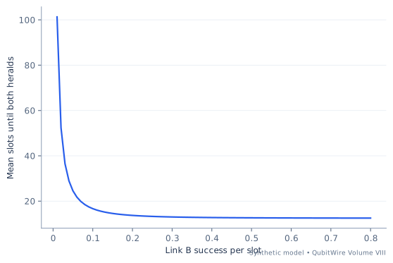
Compare the input regimes
Each case uses invented inputs. The results follow from this model and do not describe measured hardware.
Baseline regime
Complete inputs
- Link A success per slot
- 0.08
- Link B success per slot
- 0.015
- Slot duration, milliseconds
- 0.25
- The first successful link arrives with per-slot probability a + b - a b = 0.0938. Its mean wait is 10.660981 slots.
- For positive-integer geometric waits X and Y, max(X,Y) = X + Y - min(X,Y). The expected synchronized wait is 68.505686 slots.
- The earlier herald waits |X - Y| slots. Using |X-Y| = 2 max(X,Y) - X - Y gives 57.844705. Simultaneous-only operation instead waits 833.333333 slots on average.
| Calculated quantity | Synthetic result |
|---|---|
| Expected first herald, slots | 10.660980810234543 |
| Expected both heralds with perfect memory, slots | 68.50568585643212 |
| Expected age of older herald at pairing, slots | 57.844705046197575 |
| Expected simultaneous-only wait, slots | 833.3333333333334 |
| Perfect-memory mean completion, milliseconds | 17.12642146410803 |
| Simultaneous-only / memory wait | 12.164440409804177 |
Perfect storage shortens the modeled mean wait by a factor of 12.16444, but the older state waits an average of 14.461176 milliseconds. A mean age does not specify a tail probability or surviving fidelity; use the finite-memory lab when a deadline or cutoff defines usefulness.
Comparison regime
Complete inputs
- Link A success per slot
- 0.14
- Link B success per slot
- 0.055
- Slot duration, milliseconds
- 0.5
- The first successful link arrives with per-slot probability a + b - a b = 0.1873. Its mean wait is 5.339028 slots.
- For positive-integer geometric waits X and Y, max(X,Y) = X + Y - min(X,Y). The expected synchronized wait is 19.985647 slots.
- The earlier herald waits |X - Y| slots. Using |X-Y| = 2 max(X,Y) - X - Y gives 14.646619. Simultaneous-only operation instead waits 129.87013 slots on average.
| Calculated quantity | Synthetic result |
|---|---|
| Expected first herald, slots | 5.339028296849974 |
| Expected both heralds with perfect memory, slots | 19.98564702782535 |
| Expected age of older herald at pairing, slots | 14.64661873097538 |
| Expected simultaneous-only wait, slots | 129.87012987012986 |
| Perfect-memory mean completion, milliseconds | 9.992823513912676 |
| Simultaneous-only / memory wait | 6.4981698960917305 |
Perfect storage shortens the modeled mean wait by a factor of 6.49817, but the older state waits an average of 7.323309 milliseconds. A mean age does not specify a tail probability or surviving fidelity; use the finite-memory lab when a deadline or cutoff defines usefulness.
Extended regime
Complete inputs
- Link A success per slot
- 0.21200000000000002
- Link B success per slot
- 0.103
- Slot duration, milliseconds
- 0.8
- The first successful link arrives with per-slot probability a + b - a b = 0.293164. Its mean wait is 3.41106 slots.
- For positive-integer geometric waits X and Y, max(X,Y) = X + Y - min(X,Y). The expected synchronized wait is 11.014659 slots.
- The earlier herald waits |X - Y| slots. Using |X-Y| = 2 max(X,Y) - X - Y gives 7.603599. Simultaneous-only operation instead waits 45.795933 slots on average.
| Calculated quantity | Synthetic result |
|---|---|
| Expected first herald, slots | 3.41106002101213 |
| Expected both heralds with perfect memory, slots | 11.014658975141012 |
| Expected age of older herald at pairing, slots | 7.603598954128882 |
| Expected simultaneous-only wait, slots | 45.79593332112108 |
| Perfect-memory mean completion, milliseconds | 8.81172718011281 |
| Simultaneous-only / memory wait | 4.157725938177291 |
Perfect storage shortens the modeled mean wait by a factor of 4.157726, but the older state waits an average of 6.082879 milliseconds. A mean age does not specify a tail probability or surviving fidelity; use the finite-memory lab when a deadline or cutoff defines usefulness.
Try the reasoning: Why is the average age of the older herald insufficient to infer the average surviving state fidelity?
Sources and model boundaries
- RFC 9340: Architectural Principles for a Quantum Internet ↗
Quantum network architecture must account for probabilistic entanglement generation, classical coordination, memory lifetime and application requirements. Informational research guidance, not an Internet Standards Track specification or a current performance survey. The synthetic link formulas are not claims made by the RFC.
Quantum networkingThe highest delivery chance may consume too much route capacityWhich path maximizes eligible output under one shared attempt budget?
A route can be attractive for one attempt while being unattractive for the service as a whole. Additional stages may improve some component properties but consume more of a shared resource. Waiting also changes whether a delivered result remains eligible for the intended task. A useful comparison therefore names both the quality rule and the capacity denominator.
This lab uses an intentionally generic probabilistic workflow. Each candidate has a product of stage yields, a delay-dependent eligibility factor and an attempt cost proportional to its number of stages. The result with the largest per-attempt probability need not have the largest eligible output rate. All three routes are evaluated against the same total attempt-resource budget.
The abstraction is suitable for introducing a routing question, but it is not a formula for quantum entanglement quality. State fidelity does not generally multiply as these independent survival flags do. An actual quantum-network comparison must specify entanglement generation, swapping, memory, purification and scheduling. The lesson is to keep the optimization objective visible before translating a better link component into a faster useful network.
Start with the assumptions
- Stages have independent survival flags.
- The exponential term is an invented eligibility model, not fidelity.
- Every stage consumes one unit of the same attempt resource.
Eligibility probability = product(stage yields) × exp(-delay/tau)
Attempts per second = shared resource budget / stages consumed per attempt
Eligible rate = attempts per second × eligibility probability
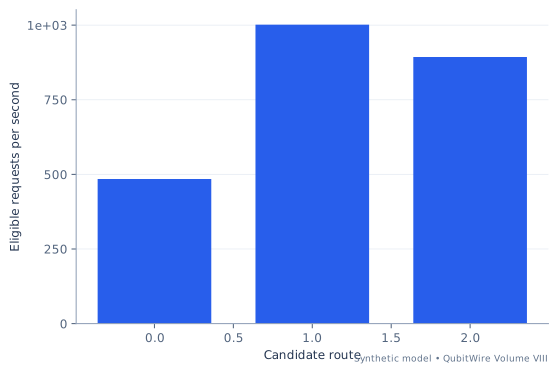
Compare the input regimes
Each case uses invented inputs. The results follow from this model and do not describe measured hardware.
Baseline regime
Complete inputs
- Eligibility decay time, milliseconds
- 5
- Attempt-resource budget per second
- 6000
- Long-route efficiency factor
- 0.8
- Direct delay, milliseconds
- 8
- Two-stage delay, milliseconds
- 3
- Three-stage delay, milliseconds
- 1.5
- Direct stage yield
- 0.4
- Two-stage yield per stage
- 0.78
- Three-stage yield per stage before efficiency factor
- 0.91
- For each candidate, multiply independent stage yields, then the declared age eligibility exp(-delay/5). This is a generic survival flag, not an entangled-state fidelity.
- Divide the shared attempt-resource budget 6,000 by the number of stages consumed per attempt. Multiplying by eligibility gives a resource-normalized rate.
- The highest rate is 1,001.690998 per second through Two stages; the highest individual-attempt eligibility belongs to Three stages.
| Calculated quantity | Synthetic result |
|---|---|
| Best rate route | Two stages |
| Best eligible rate per second | 1001.6909981988172 |
| Highest per-attempt eligibility route | Three stages |
| Direct eligible rate | 484.55164318717294 |
| Two-stage eligible rate | 1001.6909981988172 |
| Three-stage eligible rate | 893.2146038037487 |
| Route | Stages | Yield before waiting | Age eligibility factor | Eligible probability | Eligible outputs / second |
|---|---|---|---|---|---|
| Direct | 1 | 0.4 | 0.20189651799465538 | 0.08075860719786215 | 484.55164318717294 |
| Two stages | 2 | 0.6084 | 0.5488116360940264 | 0.3338969993996057 | 1001.6909981988172 |
| Three stages | 3 | 0.6028568000000001 | 0.7408182206817179 | 0.4466073019018743 | 893.2146038037487 |
A longer route can improve per-attempt delivery while consuming enough shared capacity to lose on rate. The route comparison is an original stochastic workflow abstraction. Real entanglement routing needs link scheduling, state-quality composition and correlated-resource constraints that this multiplication does not describe.
Comparison regime
Complete inputs
- Eligibility decay time, milliseconds
- 15
- Attempt-resource budget per second
- 6000
- Long-route efficiency factor
- 0.875
- Direct delay, milliseconds
- 13
- Two-stage delay, milliseconds
- 5
- Three-stage delay, milliseconds
- 2.5
- Direct stage yield
- 0.4
- Two-stage yield per stage
- 0.78
- Three-stage yield per stage before efficiency factor
- 0.91
- For each candidate, multiply independent stage yields, then the declared age eligibility exp(-delay/15). This is a generic survival flag, not an entangled-state fidelity.
- Divide the shared attempt-resource budget 6,000 by the number of stages consumed per attempt. Multiplying by eligibility gives a resource-normalized rate.
- The highest rate is 1,307.812948 per second through Two stages; the highest individual-attempt eligibility belongs to Three stages.
| Calculated quantity | Synthetic result |
|---|---|
| Best rate route | Two stages |
| Best eligible rate per second | 1307.8129480592802 |
| Highest per-attempt eligibility route | Three stages |
| Direct eligible rate | 1008.8409228208367 |
| Two-stage eligible rate | 1307.8129480592802 |
| Three-stage eligible rate | 1116.2971398382037 |
| Route | Stages | Yield before waiting | Age eligibility factor | Eligible probability | Eligible outputs / second |
|---|---|---|---|---|---|
| Direct | 1 | 0.4 | 0.4203503845086819 | 0.16814015380347277 | 1008.8409228208367 |
| Two stages | 2 | 0.6084 | 0.7165313105737893 | 0.4359376493530934 | 1307.8129480592802 |
| Three stages | 3 | 0.6593746250000001 | 0.8464817248906141 | 0.5581485699191019 | 1116.2971398382037 |
A longer route can improve per-attempt delivery while consuming enough shared capacity to lose on rate. The route comparison is an original stochastic workflow abstraction. Real entanglement routing needs link scheduling, state-quality composition and correlated-resource constraints that this multiplication does not describe.
Extended regime
Complete inputs
- Eligibility decay time, milliseconds
- 27
- Attempt-resource budget per second
- 6000
- Long-route efficiency factor
- 0.9650000000000001
- Direct delay, milliseconds
- 19
- Two-stage delay, milliseconds
- 7.4
- Three-stage delay, milliseconds
- 3.7
- Direct stage yield
- 0.4
- Two-stage yield per stage
- 0.78
- Three-stage yield per stage before efficiency factor
- 0.91
- For each candidate, multiply independent stage yields, then the declared age eligibility exp(-delay/27). This is a generic survival flag, not an entangled-state fidelity.
- Divide the shared attempt-resource budget 6,000 by the number of stages consumed per attempt. Multiplying by eligibility gives a resource-normalized rate.
- The highest rate is 1,387.655311 per second through Two stages; the highest individual-attempt eligibility belongs to Three stages.
| Calculated quantity | Synthetic result |
|---|---|
| Best rate route | Two stages |
| Best eligible rate per second | 1387.6553106767851 |
| Highest per-attempt eligibility route | Three stages |
| Direct eligible rate | 1187.398801671488 |
| Two-stage eligible rate | 1387.6553106767851 |
| Three-stage eligible rate | 1268.1395782815182 |
| Route | Stages | Yield before waiting | Age eligibility factor | Eligible probability | Eligible outputs / second |
|---|---|---|---|---|---|
| Direct | 1 | 0.4 | 0.49474950069645335 | 0.19789980027858134 | 1187.398801671488 |
| Two stages | 2 | 0.6084 | 0.7602757564523258 | 0.46255177022559507 | 1387.6553106767851 |
| Three stages | 3 | 0.7271960150000002 | 0.8719379315366007 | 0.6340697891407591 | 1268.1395782815182 |
A longer route can improve per-attempt delivery while consuming enough shared capacity to lose on rate. The route comparison is an original stochastic workflow abstraction. Real entanglement routing needs link scheduling, state-quality composition and correlated-resource constraints that this multiplication does not describe.
Try the reasoning: Which route maximizes eligibility per attempt, and which maximizes eligible output per second? Identify the shared-resource cost behind any difference.
Sources and model boundaries
- RFC 9340: Architectural Principles for a Quantum Internet ↗
Quantum network architecture must account for probabilistic entanglement generation, classical coordination, memory lifetime and application requirements. Informational research guidance, not an Internet Standards Track specification or a current performance survey. The synthetic link formulas are not claims made by the RFC.
Photonics and sensing
Photonics and sensingMore detector clicks can mean fewer clean single eventsHow many parallel channels help when the target is exactly one real signal?
Multiplexing creates more opportunities for a useful event, but it also creates more opportunities for extra signals and background clicks. Whether that is a benefit depends on the accepted event class. An experiment that needs one clean signal asks a different probability question from an experiment that counts any detector activity.
The model assigns every channel independent signal and background probabilities. It calculates exactly one signal with no backgrounds, any click of any origin, and background-only click frames. These quantities can move in different directions as more channels are added. A scan selects the largest clean-event probability within a declared range while keeping the much broader click probability visible.
The distinction is especially useful in an article about photon sources, heralded operations or detector arrays. A model can know the latent origin of every event while a real detector cannot. The clean-event calculation therefore does not assert that all clean events can be selected perfectly, or that false backgrounds can be identified in the data. That gap requires an explicit detection and validation model.
Start with the assumptions
- Signals and backgrounds are independent across and within channels.
- A frame contains one binary opportunity of each type per channel.
- Exactly one signal and no background defines the target class.
P(exactly one signal, no background) = m s (1-s)^(m-1)(1-b)^m
P(any click) = 1-(1-s)^m(1-b)^m
P(background only) = (1-s)^m[1-(1-b)^m]
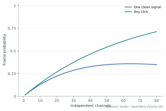
Compare the input regimes
Each case uses invented inputs. The results follow from this model and do not describe measured hardware.
Baseline regime
Complete inputs
- Signal probability per channel
- 0.015
- Background probability per channel
- 0.0005
- Maximum channels
- 80
- Frames per second
- 1000
- Exactly one signal among m independent channels has probability m s (1-s)^(m-1). Require zero independent backgrounds by multiplying by (1-b)^m.
- The scan over 1 to 80 channels peaks at m = 64, with clean-event probability 0.3588.
- Any click has probability 0.631856, which also includes unwanted multiplets and backgrounds. Background-only frames account for 1.895079% of click frames.
| Calculated quantity | Synthetic result |
|---|---|
| Best tested channel count for one clean signal | 64 |
| One-signal, no-background probability | 0.35880034788423176 |
| Any-click probability at that channel count | 0.631855893056283 |
| Background-only probability | 0.011974169898660951 |
| Background-only share of all click frames | 0.018950792467475403 |
| Clean single-signal frames per second | 358.80034788423177 |
The useful model rate is 358.800348 frames per second at 64 channels. More clicks do not necessarily mean more single-signal events. This calculation assumes the desired event class is physically meaningful; it does not assert that an ordinary detector can identify and reject every background-only frame.
Comparison regime
Complete inputs
- Signal probability per channel
- 0.045
- Background probability per channel
- 0.0025
- Maximum channels
- 80
- Frames per second
- 3500
- Exactly one signal among m independent channels has probability m s (1-s)^(m-1). Require zero independent backgrounds by multiplying by (1-b)^m.
- The scan over 1 to 80 channels peaks at m = 21, with clean-event probability 0.357002.
- Any click has probability 0.639221, which also includes unwanted multiplets and backgrounds. Background-only frames account for 3.046199% of click frames.
| Calculated quantity | Synthetic result |
|---|---|
| Best tested channel count for one clean signal | 21 |
| One-signal, no-background probability | 0.3570016568785008 |
| Any-click probability at that channel count | 0.6392205478106157 |
| Background-only probability | 0.01947193166197464 |
| Background-only share of all click frames | 0.030461992701373022 |
| Clean single-signal frames per second | 1249.5057990747528 |
The useful model rate is 1,249.505799 frames per second at 21 channels. More clicks do not necessarily mean more single-signal events. This calculation assumes the desired event class is physically meaningful; it does not assert that an ordinary detector can identify and reject every background-only frame.
Extended regime
Complete inputs
- Signal probability per channel
- 0.081
- Background probability per channel
- 0.0049
- Maximum channels
- 80
- Frames per second
- 6500
- Exactly one signal among m independent channels has probability m s (1-s)^(m-1). Require zero independent backgrounds by multiplying by (1-b)^m.
- The scan over 1 to 80 channels peaks at m = 11, with clean-event probability 0.362716.
- Any click has probability 0.625885, which also includes unwanted multiplets and backgrounds. Background-only frames account for 3.318567% of click frames.
| Calculated quantity | Synthetic result |
|---|---|
| Best tested channel count for one clean signal | 11 |
| One-signal, no-background probability | 0.3627160777397321 |
| Any-click probability at that channel count | 0.6258854372134526 |
| Background-only probability | 0.02077042648041057 |
| Background-only share of all click frames | 0.03318566824766527 |
| Clean single-signal frames per second | 2357.6545053082586 |
The useful model rate is 2,357.654505 frames per second at 11 channels. More clicks do not necessarily mean more single-signal events. This calculation assumes the desired event class is physically meaningful; it does not assert that an ordinary detector can identify and reject every background-only frame.
Try the reasoning: Why can the any-click probability keep rising after the probability of exactly one clean signal has peaked?
Neutral-atom hardware
Neutral-atom hardwareExtra loading sites help until movement becomes the limitHow many spare sites improve a complete register rather than only its initial loading?
A neutral-atom array can contain more loading sites than the final computation requires. Spares give the system a chance to select enough atoms even when individual loading is probabilistic. The relevant loading event is then at least the required number of occupied sites, rather than every site being occupied.
That change introduces a second stage. Selected atoms may need to survive movement into the target arrangement. The constructed model treats enough initial loading and survival of a fixed number of required moves as independent conditions. Increasing the number of loading sites raises the first probability while leaving the second unchanged. The result has a clear ceiling that extra empty traps cannot repair.
This simplified sequence gives readers a way to separate trap capacity, loading yield and assembled-register yield. It does not model a real rearrangement algorithm, where the number and length of moves depend on the initial pattern and many atoms may already be in useful positions. A strong follow-up article would report the distribution of loading patterns and movement costs, keeping a reliable final arrangement distinct from a large photograph of illuminated sites.
Start with the assumptions
- Sites load independently with the same probability.
- Exactly k required moves occur after successful loading.
- Movement survival is independent of loading and the other moves.
P(enough loaded) = sum_{j=k}^n C(n,j)p^j(1-p)^(n-j)
P(all required moves survive) = movement_survival^k
Assembly probability = P(enough loaded) × P(all moves survive)
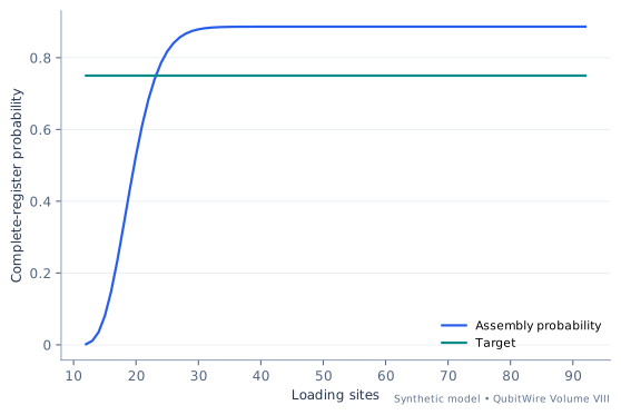
Compare the input regimes
Each case uses invented inputs. The results follow from this model and do not describe measured hardware.
Baseline regime
Complete inputs
- Required atoms
- 12
- Available loading sites
- 20
- Independent loading probability
- 0.6
- Survival per required move
- 0.99
- Desired assembled-register probability
- 0.75
- Additional sites included in search
- 80
- Sum the binomial loading distribution from 12 successes through 20. The chance of enough atoms is 0.595599.
- Assume exactly 12 independent required moves, each surviving with probability 0.99. Their joint survival is 0.886385.
- Multiply the independent loading and movement stages to obtain 0.52793. Search 12 through 92 sites for the declared target 0.75.
| Calculated quantity | Synthetic result |
|---|---|
| Probability enough atoms load | 0.5955987253122249 |
| All required moves survive | 0.8863848717161292 |
| Combined assembly probability | 0.5279296997301666 |
| No-spares complete-and-moved probability | 0.0019294669316492952 |
| Minimum sites meeting target in tested range | 24 |
| Movement-only ceiling as sites increase | 0.8863848717161292 |
The tested minimum is 24 loading sites. Extra sites fix loading shortages but cannot remove the movement ceiling 0.886385. Real rearrangement may require a variable number of moves; then its movement survival must be conditioned on the actual loading pattern.
Comparison regime
Complete inputs
- Required atoms
- 22
- Available loading sites
- 35
- Independent loading probability
- 0.725
- Survival per required move
- 0.9885
- Desired assembled-register probability
- 0.75
- Additional sites included in search
- 80
- Sum the binomial loading distribution from 22 successes through 35. The chance of enough atoms is 0.92533.
- Assume exactly 22 independent required moves, each surviving with probability 0.9885. Their joint survival is 0.77533.
- Multiply the independent loading and movement stages to obtain 0.717437. Search 22 through 102 sites for the declared target 0.75.
| Calculated quantity | Synthetic result |
|---|---|
| Probability enough atoms load | 0.925330389694105 |
| All required moves survive | 0.7753304137431637 |
| Combined assembly probability | 0.7174367938906533 |
| No-spares complete-and-moved probability | 0.0006560288895928319 |
| Minimum sites meeting target in tested range | 37 |
| Movement-only ceiling as sites increase | 0.7753304137431637 |
The tested minimum is 37 loading sites. Extra sites fix loading shortages but cannot remove the movement ceiling 0.77533. Real rearrangement may require a variable number of moves; then its movement survival must be conditioned on the actual loading pattern.
Extended regime
Complete inputs
- Required atoms
- 34
- Available loading sites
- 53
- Independent loading probability
- 0.875
- Survival per required move
- 0.9867
- Desired assembled-register probability
- 0.75
- Additional sites included in search
- 80
- Sum the binomial loading distribution from 34 successes through 53. The chance of enough atoms is 0.999997.
- Assume exactly 34 independent required moves, each surviving with probability 0.9867. Their joint survival is 0.634299.
- Multiply the independent loading and movement stages to obtain 0.634298. Search 34 through 114 sites for the declared target 0.75.
| Calculated quantity | Synthetic result |
|---|---|
| Probability enough atoms load | 0.999997255392694 |
| All required moves survive | 0.6342994851361967 |
| Combined assembly probability | 0.6342977442331956 |
| No-spares complete-and-moved probability | 0.00676968033341188 |
| Minimum sites meeting target in tested range | Target unavailable in tested range |
| Movement-only ceiling as sites increase | 0.6342994851361967 |
No tested loading-site count reaches the target. Extra sites fix loading shortages but cannot remove the movement ceiling 0.634299. Real rearrangement may require a variable number of moves; then its movement survival must be conditioned on the actual loading pattern.
Try the reasoning: Compare the desired assembly probability with the movement-only ceiling before adding more loading sites.
Hardware control and infrastructure
Hardware control and infrastructureAn idle cable can consume the margin needed to read a qubitHow does installed idle heat change the number of channels that can operate together?
More control channels appear to promise more simultaneous operations. But installed infrastructure can add a heat load even when only a subset is active. The capacity question is therefore not just the heat of the channels currently being used. It also includes the background cost of supporting every installed channel.
The lab separates fixed system heat, idle heat per installed channel and the additional heat caused by activation. The remaining budget determines how many channels can be active together. If that number is smaller than the total channel count, the readout must be scheduled in groups. A heat constraint has then become a cycle-time constraint, even though the individual readout operation is unchanged.
This is a deliberately steady-state teaching model. Real cryogenic systems have thermal time constants, frequency-dependent dissipation, unequal cable routes and temperature limits that cannot be summarized by one instantaneous wattage ceiling. The useful Model interaction is nevertheless clear: adding channels changes both available parallelism and background heat. Readers can see why a larger connector count does not, by itself, establish a proportionate increase in useful throughput.
Start with the assumptions
- Loads are modeled as steady and additive.
- Every installed channel contributes idle heat.
- Readout groups run sequentially under one heat ceiling.
Installed idle load = fixed heat + channels × idle heat
Active increment per channel = active heat - idle heat
Simultaneous capacity = floor((cooling - idle load)/active increment), capped at installed channels
Cycle time = ceil(channels/capacity) × group time + other operations
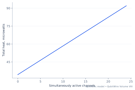
Compare the input regimes
Each case uses invented inputs. The results follow from this model and do not describe measured hardware.
Baseline regime
Complete inputs
- Installed channels
- 24
- Cooling power, microwatts
- 80
- Fixed heat, microwatts
- 20
- Idle heat per channel, microwatts
- 0.6
- Active heat per channel, microwatts
- 3
- Readout group time, microseconds
- 4
- Other cycle time, microseconds
- 12
- The installed idle load is fixed heat + channels × idle heat = 34.4 microwatts. All installed channels contribute even while their group waits.
- Each active channel adds 2.4 microwatts above that idle load. Floor the remaining margin divided by the increment, then cap at 24 installed channels.
- Read 2 groups in sequence and add other operations: 20 microseconds.
| Calculated quantity | Synthetic result |
|---|---|
| Idle installed heat, microwatts | 34.4 |
| Margin above installed idle heat | 45.6 |
| Maximum simultaneous active channels | 19 |
| Required readout groups | 2 |
| Complete cycle time, microseconds | 20 |
| All-at-once heat, microwatts | 92 |
This is a steady-load scheduling abstraction. It illustrates why additional wires can add idle heat while providing little extra simultaneous capacity. Pulsed thermal transients, unequal channels, heat sinking and maximum permissible temperatures require a real thermal analysis before applying the result to a device.
Comparison regime
Complete inputs
- Installed channels
- 44
- Cooling power, microwatts
- 100
- Fixed heat, microwatts
- 20
- Idle heat per channel, microwatts
- 0.75
- Active heat per channel, microwatts
- 3.6
- Readout group time, microseconds
- 4
- Other cycle time, microseconds
- 12
- The installed idle load is fixed heat + channels × idle heat = 53 microwatts. All installed channels contribute even while their group waits.
- Each active channel adds 2.85 microwatts above that idle load. Floor the remaining margin divided by the increment, then cap at 44 installed channels.
- Read 3 groups in sequence and add other operations: 24 microseconds.
| Calculated quantity | Synthetic result |
|---|---|
| Idle installed heat, microwatts | 53 |
| Margin above installed idle heat | 47 |
| Maximum simultaneous active channels | 16 |
| Required readout groups | 3 |
| Complete cycle time, microseconds | 24 |
| All-at-once heat, microwatts | 178.4 |
This is a steady-load scheduling abstraction. It illustrates why additional wires can add idle heat while providing little extra simultaneous capacity. Pulsed thermal transients, unequal channels, heat sinking and maximum permissible temperatures require a real thermal analysis before applying the result to a device.
Extended regime
Complete inputs
- Installed channels
- 68
- Cooling power, microwatts
- 124
- Fixed heat, microwatts
- 20
- Idle heat per channel, microwatts
- 0.9299999999999999
- Active heat per channel, microwatts
- 4.32
- Readout group time, microseconds
- 4
- Other cycle time, microseconds
- 12
- The installed idle load is fixed heat + channels × idle heat = 83.24 microwatts. All installed channels contribute even while their group waits.
- Each active channel adds 3.39 microwatts above that idle load. Floor the remaining margin divided by the increment, then cap at 68 installed channels.
- Read 6 groups in sequence and add other operations: 36 microseconds.
| Calculated quantity | Synthetic result |
|---|---|
| Idle installed heat, microwatts | 83.24 |
| Margin above installed idle heat | 40.760000000000005 |
| Maximum simultaneous active channels | 12 |
| Required readout groups | 6 |
| Complete cycle time, microseconds | 36 |
| All-at-once heat, microwatts | 313.76 |
This is a steady-load scheduling abstraction. It illustrates why additional wires can add idle heat while providing little extra simultaneous capacity. Pulsed thermal transients, unequal channels, heat sinking and maximum permissible temperatures require a real thermal analysis before applying the result to a device.
Try the reasoning: What happens to idle heat and simultaneous capacity when more channels are installed? Check both before using the cycle-time estimate.
Sources and model boundaries
- A Quantum Engineer's Guide to Superconducting Qubits ↗
Superconducting qubit engineering links device physics, noise, control and measurement infrastructure. No contemporary device specification, operating temperature, pulse duration or thermal budget is inferred from this historical review.
Hardware control and infrastructureReadout can move its bottleneck without changing the detectorWhat is gained when acquisition, transfer and processing overlap?
A measurement can produce far more data than the final bit returned to an application. Raw waveforms may support discrimination, calibration and diagnostics, while the later result contains only a compact decision. The complete readout workflow therefore includes acquisition, transport and processing resources with different timing and storage needs.
A sequential schedule pays all three stage times for every shot. A perfectly overlapped pipeline pays the fill cost once and then completes shots at the pace of the slowest stage. Improving a stage that is already faster than the bottleneck may have little effect on sustained throughput. Reducing raw data near the detector can alter the transfer requirement, but it may also discard information useful for auditing a classifier.
The cases calculate byte counts and batch durations under explicit decimal bandwidth units. The pipeline is idealized: stages have separate resources and there is no feedback dependence between consecutive shots. Those assumptions are often the first thing to examine in a mid-circuit-control claim. A result that depends on the previous measurement cannot automatically receive the same overlap as an independent batch of final readouts.
Start with the assumptions
- Stages have dedicated resources and sufficient buffers.
- All shots have identical stage durations.
- Consecutive shots are independent for scheduling purposes.
Raw bytes = channels × samples per channel × bytes per complex sample
Transfer time = raw bytes / transfer bandwidth
Serial batch = N × sum(stage times)
Ideal pipeline batch = sum(stage times) + (N-1) × max(stage times)
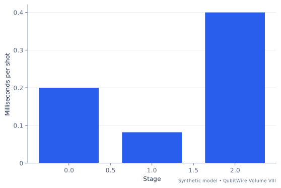
Compare the input regimes
Each case uses invented inputs. The results follow from this model and do not describe measured hardware.
Baseline regime
Complete inputs
- Readout channels
- 8
- Samples per channel
- 512
- Bytes per complex sample
- 4
- Transfer bandwidth, MB per second
- 200
- Feature extraction, milliseconds
- 0.4
- Acquisition, milliseconds
- 0.2
- Shots in batch
- 1000
- Multiply channels × samples × bytes per complex sample to obtain 16,384 raw bytes. MB uses 1,000,000 bytes in this case.
- Divide by link bandwidth: transfer requires 0.08192 milliseconds per shot. The other stage times are 0.2 and 0.4 milliseconds.
- A perfectly overlapped three-stage pipeline fills once, then completes one shot per slowest-stage interval. Total = sum(stage times) + (shots - 1) × max(stage times) = 0.400282 seconds.
| Calculated quantity | Synthetic result |
|---|---|
| Raw bytes per shot | 16384 |
| Transfer time per shot, milliseconds | 0.08192 |
| Serial batch duration, seconds | 0.6819200000000001 |
| Ideal pipeline batch duration, seconds | 0.40028192 |
| Raw bytes / one-bit-per-channel result bytes | 16384 |
| Pipeline limiting stage, milliseconds | 0.4 |
The pipeline model shortens this batch from 0.68192 to 0.400282 seconds. It assumes distinct resources, sufficient buffers and no next-shot dependence on the previous result. Mid-circuit feedback can impose dependencies that prevent this overlap. A compressed result may omit waveform information needed for later calibration checks.
Comparison regime
Complete inputs
- Readout channels
- 28
- Samples per channel
- 640
- Bytes per complex sample
- 4
- Transfer bandwidth, MB per second
- 250
- Feature extraction, milliseconds
- 0.65
- Acquisition, milliseconds
- 0.25
- Shots in batch
- 1000
- Multiply channels × samples × bytes per complex sample to obtain 71,680 raw bytes. MB uses 1,000,000 bytes in this case.
- Divide by link bandwidth: transfer requires 0.28672 milliseconds per shot. The other stage times are 0.25 and 0.65 milliseconds.
- A perfectly overlapped three-stage pipeline fills once, then completes one shot per slowest-stage interval. Total = sum(stage times) + (shots - 1) × max(stage times) = 0.650537 seconds.
| Calculated quantity | Synthetic result |
|---|---|
| Raw bytes per shot | 71680 |
| Transfer time per shot, milliseconds | 0.28672000000000003 |
| Serial batch duration, seconds | 1.18672 |
| Ideal pipeline batch duration, seconds | 0.6505367200000001 |
| Raw bytes / one-bit-per-channel result bytes | 20480 |
| Pipeline limiting stage, milliseconds | 0.65 |
The pipeline model shortens this batch from 1.18672 to 0.650537 seconds. It assumes distinct resources, sufficient buffers and no next-shot dependence on the previous result. Mid-circuit feedback can impose dependencies that prevent this overlap. A compressed result may omit waveform information needed for later calibration checks.
Extended regime
Complete inputs
- Readout channels
- 52
- Samples per channel
- 896
- Bytes per complex sample
- 4
- Transfer bandwidth, MB per second
- 250
- Feature extraction, milliseconds
- 0.9500000000000001
- Acquisition, milliseconds
- 0.31
- Shots in batch
- 1000
- Multiply channels × samples × bytes per complex sample to obtain 186,368 raw bytes. MB uses 1,000,000 bytes in this case.
- Divide by link bandwidth: transfer requires 0.745472 milliseconds per shot. The other stage times are 0.31 and 0.95 milliseconds.
- A perfectly overlapped three-stage pipeline fills once, then completes one shot per slowest-stage interval. Total = sum(stage times) + (shots - 1) × max(stage times) = 0.951055 seconds.
| Calculated quantity | Synthetic result |
|---|---|
| Raw bytes per shot | 186368 |
| Transfer time per shot, milliseconds | 0.7454719999999999 |
| Serial batch duration, seconds | 2.005472 |
| Ideal pipeline batch duration, seconds | 0.9510554720000001 |
| Raw bytes / one-bit-per-channel result bytes | 28672 |
| Pipeline limiting stage, milliseconds | 0.9500000000000001 |
The pipeline model shortens this batch from 2.005472 to 0.951055 seconds. It assumes distinct resources, sufficient buffers and no next-shot dependence on the previous result. Mid-circuit feedback can impose dependencies that prevent this overlap. A compressed result may omit waveform information needed for later calibration checks.
Try the reasoning: Which stage would need to be faster to improve steady pipeline throughput? Would a next-shot feedback dependency allow the same overlap?
Sources and model boundaries
- A Quantum Engineer's Guide to Superconducting Qubits ↗
Superconducting qubit engineering links device physics, noise, control and measurement infrastructure. No contemporary device specification, operating temperature, pulse duration or thermal budget is inferred from this historical review.
Hardware control and infrastructureQuieting a microwave line also decides where heat appearsHow does distributing attenuation change thermal occupation and signal dissipation?
An attenuator reduces a traveling signal but also couples the line to its own environment. At microwave frequencies, a temperature is most useful when compared with the mode’s quantum energy scale. The mean thermal occupation expresses that relationship and lets a simple matched-loss model track noise through successive stages.
Each ideal stage transmits a fraction of the incoming occupation and replaces the lost fraction with its own thermal contribution. Moving attenuation between warmer and colder stages therefore changes which environment dominates the output. The same distribution also determines where incident classical signal power is dissipated. A quiet output and a manageable cold-stage heat load are related but distinct objectives.
The lab tracks two stages using invented attenuation values and temperatures. It explicitly balances only the declared incident signal power, not every thermal pathway in a refrigerator. Broadband radiation, cable conduction, reflections, filters and nonlinearity are omitted. The result is appropriate as a Model explanation of why control wiring is engineered in stages, while remaining far narrower than a design for an operating quantum processor.
Start with the assumptions
- One bosonic mode and ideal matched linear attenuation are modeled.
- Each attenuator has a fixed temperature.
- The stated power balance concerns only incident classical signal power.
Thermal occupation n(T) = 1/[exp(h f/(k_B T))-1]
Power transmission eta = 10^(-attenuation_dB/10)
Matched-stage occupation n_out = eta n_in + (1-eta)n_stage
Signal dissipation = incident signal power × (1-eta)
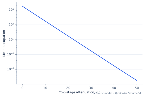
Compare the input regimes
Each case uses invented inputs. The results follow from this model and do not describe measured hardware.
Baseline regime
Complete inputs
- Mode frequency, GHz
- 4
- Input temperature, K
- 300
- Warm-stage attenuation, dB
- 10
- Cold-stage attenuation, dB
- 30
- Warm-stage temperature, K
- 4
- Cold-stage temperature, K
- 0.02
- Incident signal power, microwatts
- 10
- Planck constant / Boltzmann constant, K seconds
- 4.799243073e-11
- For one bosonic mode, n(T) = 1/(exp(h f / kT) - 1). The stipulated input temperature gives occupation 1,562.246488.
- Each ideal matched attenuator mixes transmitted input noise with its own thermal noise: n_out = eta n_in + (1 - eta)n_stage. The two stages give 174.531205 and 0.174599.
- Classical incident signal power dissipates as P_in(1 - eta) at each stage, after accounting for preceding attenuation. The signal-power balance sums to 10 microwatts.
| Calculated quantity | Synthetic result |
|---|---|
| Incoming mean thermal occupation | 1562.2464876937408 |
| After warm stage occupation | 174.53120527593762 |
| After cold stage occupation | 0.1745989733869517 |
| Warm-stage signal dissipation, microwatts | 9 |
| Cold-stage signal dissipation, microwatts | 0.999 |
| Remaining signal power, microwatts | 0.001 |
Moving attenuation changes both the final noise occupation and where the signal power is dissipated. This calculation accounts only for the declared traveling mode and incident signal. It omits reflections, broadband thermal transport, cable conduction and nonlinear components, so it is an explanatory balance rather than a refrigerator wiring design.
Comparison regime
Complete inputs
- Mode frequency, GHz
- 5
- Input temperature, K
- 300
- Warm-stage attenuation, dB
- 20
- Cold-stage attenuation, dB
- 20
- Warm-stage temperature, K
- 4
- Cold-stage temperature, K
- 0.025
- Incident signal power, microwatts
- 15
- Planck constant / Boltzmann constant, K seconds
- 4.799243073e-11
- For one bosonic mode, n(T) = 1/(exp(h f / kT) - 1). The stipulated input temperature gives occupation 1,249.697214.
- Each ideal matched attenuator mixes transmitted input noise with its own thermal noise: n_out = eta n_in + (1 - eta)n_stage. The two stages give 28.509523 and 0.285162.
- Classical incident signal power dissipates as P_in(1 - eta) at each stage, after accounting for preceding attenuation. The signal-power balance sums to 15 microwatts.
| Calculated quantity | Synthetic result |
|---|---|
| Incoming mean thermal occupation | 1249.6972141512078 |
| After warm stage occupation | 28.509523411031747 |
| After cold stage occupation | 0.2851623916978089 |
| Warm-stage signal dissipation, microwatts | 14.85 |
| Cold-stage signal dissipation, microwatts | 0.1485 |
| Remaining signal power, microwatts | 0.0015 |
Moving attenuation changes both the final noise occupation and where the signal power is dissipated. This calculation accounts only for the declared traveling mode and incident signal. It omits reflections, broadband thermal transport, cable conduction and nonlinear components, so it is an explanatory balance rather than a refrigerator wiring design.
Extended regime
Complete inputs
- Mode frequency, GHz
- 6.2
- Input temperature, K
- 300
- Warm-stage attenuation, dB
- 32
- Cold-stage attenuation, dB
- 8
- Warm-stage temperature, K
- 4
- Cold-stage temperature, K
- 0.031
- Incident signal power, microwatts
- 21
- Planck constant / Boltzmann constant, K seconds
- 4.799243073e-11
- For one bosonic mode, n(T) = 1/(exp(h f / kT) - 1). The stipulated input temperature gives occupation 1,007.723589.
- Each ideal matched attenuator mixes transmitted input noise with its own thermal noise: n_out = eta n_in + (1 - eta)n_stage. The two stages give 13.576839 and 2.151841.
- Classical incident signal power dissipates as P_in(1 - eta) at each stage, after accounting for preceding attenuation. The signal-power balance sums to 21 microwatts.
| Calculated quantity | Synthetic result |
|---|---|
| Incoming mean thermal occupation | 1007.7235886980283 |
| After warm stage occupation | 13.576838751448957 |
| After cold stage occupation | 2.1518410159052763 |
| Warm-stage signal dissipation, microwatts | 20.986749895765918 |
| Cold-stage signal dissipation, microwatts | 0.011150104234084053 |
| Remaining signal power, microwatts | 0.002099999999999999 |
Moving attenuation changes both the final noise occupation and where the signal power is dissipated. This calculation accounts only for the declared traveling mode and incident signal. It omits reflections, broadband thermal transport, cable conduction and nonlinear components, so it is an explanatory balance rather than a refrigerator wiring design.
Try the reasoning: Move attenuation between the warm and cold stages while keeping total decibels fixed. Track both output occupation and the location of signal dissipation.
Sources and model boundaries
- A Quantum Engineer's Guide to Superconducting Qubits ↗
Superconducting qubit engineering links device physics, noise, control and measurement infrastructure. No contemporary device specification, operating temperature, pulse duration or thermal budget is inferred from this historical review.
Simulation and scientific validity
Simulation and scientific validityA neat finite-size fit can point to the wrong limitWhat does a held-out size reveal that an in-sample residual cannot?
A finite quantum simulator answers a finite question. Researchers may then ask how the observable changes as the represented system becomes larger. Extrapolation can be informative, but the inferred limit depends on a functional form and a range of sizes. A narrow fitted residual is evidence about the observed window, not automatic evidence about an unobserved limit.
This lab creates an exact curve with both inverse-size and inverse-size-squared terms. It deliberately fits only the first term. Because the generating limit is known, the error in the extrapolated intercept is visible. Comparing all sizes with the largest two, and testing a new holdout size, reveals sensitivity that the fitted line alone could conceal.
The example avoids simulated measurement noise so the source of error stays clear: the model is misspecified. In a real study, sampling noise, control error and different finite-size corrections can coexist. Comparing fit windows alongside explicit extrapolation assumptions exposes this sensitivity. Readers should be able to distinguish a directly measured finite-size observable from an inferred large-system value.
Start with the assumptions
- The generating curve is known only because this is synthetic.
- Fits use exact values without measurement noise.
- Ordinary least squares weights all supplied sizes equally.
Synthetic observable y(L) = y_infinity + a/L + b/L²
Deliberately restricted fit y_fit(L) = intercept + slope/L
Holdout error = fitted prediction at unused size - generating value
Compare the input regimes
Each case uses invented inputs. The results follow from this model and do not describe measured hardware.
Baseline regime
Complete inputs
- Infinite-size reference
- 0.6
- Inverse-size coefficient
- 1.5
- Curvature coefficient
- 2
- System sizes
- 6, 10, 16, 24
- Unfitted holdout size
- 40
- Generate y(L) = reference + a/L + b/L² at L = 6, 10, 16, 24. These are exact synthetic function values, not noisy observations.
- Fit a straight line in 1/L while omitting curvature. Using all sizes gives intercept 0.582319; the largest two give 0.594792.
- At the held-out size 40, the all-size fit predicts 0.630441 and the generating curve gives 0.63875. Their difference is -0.008309.
| Calculated quantity | Synthetic result |
|---|---|
| All-size linear extrapolated intercept | 0.5823186709873579 |
| Largest-two extrapolated intercept | 0.5947916666666666 |
| Known synthetic infinite-size reference | 0.6 |
| All-size intercept bias | -0.017681329012642077 |
| In-sample residual RMS | 0.003240669796073463 |
| Unfitted holdout prediction minus truth | -0.008308929428708534 |
| System size | Observable |
|---|---|
| 6 | 0.9055555555555556 |
| 10 | 0.77 |
| 16 | 0.7015625 |
| 24 | 0.6659722222222222 |
The known intercept is 0.6, so the fitted intercept error can be measured directly here. A small residual over the observed window does not guarantee an accurate extrapolation outside it. On a real experiment the infinite-size answer is unknown; varying the fit window and testing held-out sizes becomes evidence about model sensitivity, not proof of the limit.
Comparison regime
Complete inputs
- Infinite-size reference
- 0.65
- Inverse-size coefficient
- 1.1
- Curvature coefficient
- 8
- System sizes
- 11, 15, 21, 29
- Unfitted holdout size
- 50
- Generate y(L) = reference + a/L + b/L² at L = 11, 15, 21, 29. These are exact synthetic function values, not noisy observations.
- Fit a straight line in 1/L while omitting curvature. Using all sizes gives intercept 0.621764; the largest two give 0.636864.
- At the held-out size 50, the all-size fit predicts 0.66398 and the generating curve gives 0.6752. Their difference is -0.01122.
| Calculated quantity | Synthetic result |
|---|---|
| All-size linear extrapolated intercept | 0.6217640825006453 |
| Largest-two extrapolated intercept | 0.6368637110016419 |
| Known synthetic infinite-size reference | 0.65 |
| All-size intercept bias | -0.028235917499354724 |
| In-sample residual RMS | 0.0027585201551087405 |
| Unfitted holdout prediction minus truth | -0.01121975718117707 |
| System size | Observable |
|---|---|
| 11 | 0.8161157024793388 |
| 15 | 0.758888888888889 |
| 21 | 0.7205215419501134 |
| 29 | 0.6974435196195006 |
The known intercept is 0.65, so the fitted intercept error can be measured directly here. A small residual over the observed window does not guarantee an accurate extrapolation outside it. On a real experiment the infinite-size answer is unknown; varying the fit window and testing held-out sizes becomes evidence about model sensitivity, not proof of the limit.
Extended regime
Complete inputs
- Infinite-size reference
- 0.71
- Inverse-size coefficient
- 0.62
- Curvature coefficient
- 15.2
- System sizes
- 17, 21, 27, 35
- Unfitted holdout size
- 62
- Generate y(L) = reference + a/L + b/L² at L = 17, 21, 27, 35. These are exact synthetic function values, not noisy observations.
- Fit a straight line in 1/L while omitting curvature. Using all sizes gives intercept 0.682791; the largest two give 0.693915.
- At the held-out size 62, the all-size fit predicts 0.714273 and the generating curve gives 0.723954. Their difference is -0.009681.
| Calculated quantity | Synthetic result |
|---|---|
| All-size linear extrapolated intercept | 0.6827909087164262 |
| Largest-two extrapolated intercept | 0.6939153439153434 |
| Known synthetic infinite-size reference | 0.71 |
| All-size intercept bias | -0.02720909128357374 |
| In-sample residual RMS | 0.0015193266736859916 |
| Unfitted holdout prediction minus truth | -0.009680813148590484 |
| System size | Observable |
|---|---|
| 17 | 0.7990657439446367 |
| 21 | 0.7739909297052153 |
| 27 | 0.7538134430727023 |
| 35 | 0.7401224489795918 |
The known intercept is 0.71, so the fitted intercept error can be measured directly here. A small residual over the observed window does not guarantee an accurate extrapolation outside it. On a real experiment the infinite-size answer is unknown; varying the fit window and testing held-out sizes becomes evidence about model sensitivity, not proof of the limit.
Try the reasoning: Can a two-point fit with zero residual certify the infinite-size limit? Compare the fit-window change and the held-out-size error.
Simulation and scientific validityMore simulation steps can improve the formula and worsen the experimentWhere is the optimum when approximation error falls while implementation error grows?
Splitting an evolution into more steps can make a product-formula approximation more faithful to the target mathematical evolution. The implementation then performs more operations, each of which may introduce error or consume resources. A step count therefore sits between two models: the mathematical approximation and the physical realization.
The deliberately simple objective in this lab contains one term that falls as an inverse power of the step count and one that grows linearly. Its continuous minimum can be derived by differentiation, then compared with the allowed integers. Both contributions remain visible. This prevents a decreasing approximation bound from being mistaken for a decreasing total experimental error.
The cited product-formula work supplies the context that approximation error depends on mathematical structure. It does not supply this toy model’s coefficients or certify that a linear implementation term is appropriate. Before applying the sum to a real experiment, the two contributions would need compatible units and an error measure for which the combination is justified. Changing the step count is meaningful only while those model assumptions remain appropriate.
Start with the assumptions
- The two contributions share a compatible illustrative error measure.
- Coefficients are positive and fixed.
- The implementation term is assumed linear for teaching purposes.
Illustrative error objective E(r) = a/r^q + b r
Continuous stationary point r* = (q a/b)^(1/(q+1))
Integer optimum is selected from the stated finite step range
Compare the input regimes
Each case uses invented inputs. The results follow from this model and do not describe measured hardware.
Baseline regime
Complete inputs
- Approximation coefficient
- 0.4
- Error added per step
- 0.0002
- Inverse-step power
- 1
- Maximum steps
- 120
- The deliberately assumed objective is a/r^q + b r. Differentiate: -q a/r^(q+1) + b = 0, giving r* = 44.72136.
- Scan positive integers up to 120. The minimum occurs at r = 45, where the terms are 0.008889 and 0.009.
- The summed quantity is an illustrative error objective. Its coefficients must refer to a compatible error measure before terms can be physically added. It is not a general Trotter bound for an arbitrary Hamiltonian.
| Calculated quantity | Synthetic result |
|---|---|
| Continuous unconstrained optimum | 44.721359549995796 |
| Best tested integer step count | 45 |
| Approximation contribution at optimum | 0.008888888888888889 |
| Implementation contribution at optimum | 0.009000000000000001 |
| Combined illustrative error objective | 0.01788888888888889 |
| One-step objective / best objective | 22.371428571428567 |
The numerical optimum is 45 steps. Increasing steps beyond it reduces one term while increasing the other. The cited product-formula literature motivates the existence of approximation error, but the additive linear implementation term and all coefficients are assumptions created for this decision exercise.
Comparison regime
Complete inputs
- Approximation coefficient
- 0.9
- Error added per step
- 0.0007
- Inverse-step power
- 2
- Maximum steps
- 120
- The deliberately assumed objective is a/r^q + b r. Differentiate: -q a/r^(q+1) + b = 0, giving r* = 13.700134.
- Scan positive integers up to 120. The minimum occurs at r = 14, where the terms are 0.004592 and 0.0098.
- The summed quantity is an illustrative error objective. Its coefficients must refer to a compatible error measure before terms can be physically added. It is not a general Trotter bound for an arbitrary Hamiltonian.
| Calculated quantity | Synthetic result |
|---|---|
| Continuous unconstrained optimum | 13.700134211888825 |
| Best tested integer step count | 14 |
| Approximation contribution at optimum | 0.004591836734693878 |
| Implementation contribution at optimum | 0.0098 |
| Combined illustrative error objective | 0.014391836734693877 |
| One-step objective / best objective | 62.58408961996597 |
The numerical optimum is 14 steps. Increasing steps beyond it reduces one term while increasing the other. The cited product-formula literature motivates the existence of approximation error, but the additive linear implementation term and all coefficients are assumptions created for this decision exercise.
Extended regime
Complete inputs
- Approximation coefficient
- 1.5
- Error added per step
- 0.0013000000000000002
- Inverse-step power
- 2
- Maximum steps
- 120
- The deliberately assumed objective is a/r^q + b r. Differentiate: -q a/r^(q+1) + b = 0, giving r* = 13.214761.
- Scan positive integers up to 120. The minimum occurs at r = 13, where the terms are 0.008876 and 0.0169.
- The summed quantity is an illustrative error objective. Its coefficients must refer to a compatible error measure before terms can be physically added. It is not a general Trotter bound for an arbitrary Hamiltonian.
| Calculated quantity | Synthetic result |
|---|---|
| Continuous unconstrained optimum | 13.214760630124598 |
| Best tested integer step count | 13 |
| Approximation contribution at optimum | 0.008875739644970414 |
| Implementation contribution at optimum | 0.016900000000000002 |
| Combined illustrative error objective | 0.025775739644970416 |
| One-step objective / best objective | 58.24469135235646 |
The numerical optimum is 13 steps. Increasing steps beyond it reduces one term while increasing the other. The cited product-formula literature motivates the existence of approximation error, but the additive linear implementation term and all coefficients are assumptions created for this decision exercise.
Try the reasoning: At the continuous stationary point, what relation holds between the approximation and implementation terms for inverse-step power q?
Sources and model boundaries
- A Theory of Trotter Error ↗
Product-formula approximation error depends on the mathematical structure of Hamiltonian terms. The lab does not reproduce a paper benchmark or a Hamiltonian-specific bound. Its additive implementation-error term is a teaching assumption.
Simulation and scientific validityA perfect sampled fit can describe the wrong oscillationCan two different continuous frequencies produce the same recorded values?
An oscilloscope or software logger records samples, not an unbroken view of a waveform. Different continuous signals can agree at those sample times. If an analysis chooses between them only by how well it fits the recorded values, it can have no basis for preferring the physically correct one.
The constructed experiment samples a zero-phase cosine at a fixed rate. Folding its frequency into the base interval gives an alias with the same ideal sample sequence. The numerical comparison makes the ambiguity concrete: two plotted continuous explanations can diverge between sample times while their recorded points coincide. More elaborate fitting does not recover information that the measurement procedure never distinguished.
This lesson applies to control waveforms, spectroscopy traces and simulated dynamics. A justified bandwidth limit, anti-alias filtering or a changed sampling schedule can supply the missing constraint. The example also distinguishes Fourier-bin spacing from a universal resolution claim. A longer record changes the analysis grid, but identifiability still depends on the signal model, window and measurement process.
Start with the assumptions
- The signal is a zero-phase cosine with a known fixed amplitude.
- Sampling is exact and uniformly spaced.
- Floating-point discrepancies are numerical error, not physical noise.
Samples occur at t_k = k/f_s
Cosine alias = |((f+f_s/2) modulo f_s)-f_s/2|
DFT-bin spacing = f_s/N
Compare the input regimes
Each case uses invented inputs. The results follow from this model and do not describe measured hardware.
Baseline regime
Complete inputs
- Sampling rate, Hz
- 80
- Actual sinusoid frequency, Hz
- 91
- Sample count
- 32
- Signal amplitude
- 1
- Fold the actual frequency into the interval from zero to fs/2: |((f + fs/2) mod fs) - fs/2| = 11 Hz.
- Evaluate zero-phase cosines at t_k = k/fs for k = 0,...,31. The largest difference between actual and aliased sample values is 2.29816e-14, arising from floating-point arithmetic.
- The spacing of the discrete Fourier transform bins is fs/N = 2.5 Hz. This is a grid spacing, not a universal resolution limit or a proof that adjacent lines are separable.
| Calculated quantity | Synthetic result |
|---|---|
| Folded alias frequency, Hz | 11 |
| Sampling Nyquist boundary, Hz | 40 |
| Observation duration N/fs, seconds | 0.4 |
| DFT-bin spacing fs/N, Hz | 2.5 |
| Maximum numerical sample discrepancy | 2.298161660974074e-14 |
| Index | Time, seconds | Actual-frequency sample | Alias-frequency sample |
|---|---|---|---|
| 0 | 0 | 1 | 1 |
| 1 | 0.0125 | 0.6494480483301835 | 0.6494480483301837 |
| 2 | 0.025 | -0.1564344650402312 | -0.1564344650402308 |
| 3 | 0.0375 | -0.8526401643540921 | -0.852640164354092 |
| 4 | 0.05 | -0.9510565162951534 | -0.9510565162951536 |
| 5 | 0.0625 | -0.38268343236509145 | -0.38268343236509034 |
| 6 | 0.075 | 0.4539904997395461 | 0.4539904997395458 |
| 7 | 0.0875 | 0.972369920397675 | 0.9723699203976762 |
| 8 | 0.1 | 0.8090169943749467 | 0.8090169943749476 |
| 9 | 0.1125 | 0.07845909572784966 | 0.07845909572784569 |
| 10 | 0.125 | -0.7071067811865449 | -0.7071067811865467 |
| 11 | 0.1375 | -0.9969173337331282 | -0.996917333733128 |
The 91 Hz and 11 Hz zero-phase cosines give the same ideal sample sequence. A better-fitting sampled curve cannot identify which continuous signal was present. Filtering, an independently justified bandwidth limit or a changed sampling rate supplies information absent from the original samples.
Comparison regime
Complete inputs
- Sampling rate, Hz
- 130
- Actual sinusoid frequency, Hz
- 281
- Sample count
- 40
- Signal amplitude
- 1.5
- Fold the actual frequency into the interval from zero to fs/2: |((f + fs/2) mod fs) - fs/2| = 21 Hz.
- Evaluate zero-phase cosines at t_k = k/fs for k = 0,...,39. The largest difference between actual and aliased sample values is 1.00031e-13, arising from floating-point arithmetic.
- The spacing of the discrete Fourier transform bins is fs/N = 3.25 Hz. This is a grid spacing, not a universal resolution limit or a proof that adjacent lines are separable.
| Calculated quantity | Synthetic result |
|---|---|
| Folded alias frequency, Hz | 21 |
| Sampling Nyquist boundary, Hz | 65 |
| Observation duration N/fs, seconds | 0.3076923076923077 |
| DFT-bin spacing fs/N, Hz | 3.25 |
| Maximum numerical sample discrepancy | 1.000310945187266e-13 |
| Index | Time, seconds | Actual-frequency sample | Alias-frequency sample |
|---|---|---|---|
| 0 | 0 | 1.5 | 1.5 |
| 1 | 0.007692307692307693 | 0.7914603661592006 | 0.791460366159199 |
| 2 | 0.015384615384615385 | -0.6647873183988586 | -0.6647873183988624 |
| 3 | 0.023076923076923078 | -1.4929974520764726 | -1.492997452076473 |
| 4 | 0.03076923076923077 | -0.9107437617280726 | -0.910743761728066 |
| 5 | 0.038461538461538464 | 0.5319073305637925 | 0.5319073305638033 |
| 6 | 0.046153846153846156 | 1.4720551892091192 | 1.47205518920912 |
| 7 | 0.05384615384615385 | 1.0215237881801953 | 1.0215237881801955 |
| 8 | 0.06153846153846154 | -0.3940610672978664 | -0.39406106729788226 |
| 9 | 0.06923076923076923 | -1.4373687436637468 | -1.4373687436637494 |
| 10 | 0.07692307692307693 | -1.1227661222566674 | -1.1227661222566518 |
| 11 | 0.08461538461538462 | 0.2525355620205407 | 0.2525355620205592 |
The 281 Hz and 21 Hz zero-phase cosines give the same ideal sample sequence. A better-fitting sampled curve cannot identify which continuous signal was present. Filtering, an independently justified bandwidth limit or a changed sampling rate supplies information absent from the original samples.
Extended regime
Complete inputs
- Sampling rate, Hz
- 190
- Actual sinusoid frequency, Hz
- 413
- Sample count
- 40
- Signal amplitude
- 2.1
- Fold the actual frequency into the interval from zero to fs/2: |((f + fs/2) mod fs) - fs/2| = 33 Hz.
- Evaluate zero-phase cosines at t_k = k/fs for k = 0,...,39. The largest difference between actual and aliased sample values is 9.54792e-14, arising from floating-point arithmetic.
- The spacing of the discrete Fourier transform bins is fs/N = 4.75 Hz. This is a grid spacing, not a universal resolution limit or a proof that adjacent lines are separable.
| Calculated quantity | Synthetic result |
|---|---|
| Folded alias frequency, Hz | 33 |
| Sampling Nyquist boundary, Hz | 95 |
| Observation duration N/fs, seconds | 0.21052631578947367 |
| DFT-bin spacing fs/N, Hz | 4.75 |
| Maximum numerical sample discrepancy | 9.547918011776346e-14 |
| Index | Time, seconds | Actual-frequency sample | Alias-frequency sample |
|---|---|---|---|
| 0 | 0 | 2.1 | 2.1 |
| 1 | 0.005263157894736842 | 0.9688164422552462 | 0.9688164422552444 |
| 2 | 0.010526315789473684 | -1.2060901916341784 | -1.2060901916341815 |
| 3 | 0.015789473684210527 | -2.0816545455866473 | -2.081654545586648 |
| 4 | 0.021052631578947368 | -0.7146156663274583 | -0.714615666327451 |
| 5 | 0.02631578947368421 | 1.4222913004140512 | 1.4222913004140565 |
| 6 | 0.031578947368421054 | 2.0269387115824298 | 2.026938711582432 |
| 7 | 0.03684210526315789 | 0.44792922456190093 | 0.44792922456187023 |
| 8 | 0.042105263157894736 | -1.6136423327993934 | -1.6136423327994034 |
| 9 | 0.04736842105263158 | -1.936808485452508 | -1.9368084854525074 |
| 10 | 0.05263157894736842 | -0.1734166254919114 | -0.17341662549189743 |
| 11 | 0.05789473684210526 | 1.7768000300839661 | 1.7768000300839641 |
The 413 Hz and 33 Hz zero-phase cosines give the same ideal sample sequence. A better-fitting sampled curve cannot identify which continuous signal was present. Filtering, an independently justified bandwidth limit or a changed sampling rate supplies information absent from the original samples.
Try the reasoning: How would a second sampling rate or a verified analog bandwidth limit distinguish the continuous frequencies that share these samples?
Simulation and scientific validityOne more checkpoint can remove a whole parallel jobHow do memory boundaries change a simulator batch schedule?
Classical simulation resources grow rapidly with the number of represented qubits, but a state-vector size is only the start of memory accounting. Workspaces, snapshots and concurrent jobs compete for the same allocation. A modest extra resident buffer can push a job across a discrete concurrency boundary.
The lab budgets a dense complex128 state, a workspace factor and a declared number of resident checkpoint copies. It then floors available RAM divided by the complete per-job footprint. The number of waves needed to complete a batch can jump even when the footprint changes smoothly. A save-time cost adds a second effect that is kept separate from the lost parallel capacity.
Checkpointing can still be valuable because it protects work against failures. The no-failure schedule here deliberately does not assign that benefit a made-up value. A complete decision would model checkpoint location, restart frequency, save duration and recovery time. The existing state-vector calculator can use this example as an extension from abstract storage growth to a realistic question about which resources must coexist.
Start with the assumptions
- Checkpoints are additional resident full-state copies.
- All jobs take the same time and can run independently.
- No failures occur during this schedule comparison.
Dense complex128 state bytes = 16 × 2^qubits
Resident job GiB = state_GiB × (workspace factor + checkpoint copies)
Concurrency = floor(available_GiB / job_GiB)
Batch time = ceil(jobs/concurrency) × (base runtime + checkpoint-save time)
Compare the input regimes
Each case uses invented inputs. The results follow from this model and do not describe measured hardware.
Baseline regime
Complete inputs
- Simulated qubits
- 24
- Available RAM, GiB
- 64
- Workspace factor
- 1.5
- Checkpoint copies per job
- 1
- Independent jobs
- 24
- Base runtime per job, seconds
- 20
- Save time per checkpoint, seconds
- 2
- Complex128 amplitudes use 16 × 2^24 bytes = 0.25 GiB. A GiB is 2^30 bytes.
- Workspace plus resident checkpoint copies multiply that state footprint by 2.5, giving 0.625 GiB per job. Floor available RAM divided by that footprint.
- The 24 jobs require 1 waves, each taking 22 seconds.
| Calculated quantity | Synthetic result |
|---|---|
| Dense state-vector memory, GiB | 0.25 |
| Memory per checkpointed job, GiB | 0.625 |
| Checkpointed concurrent jobs | 102 |
| Checkpointed batch duration, seconds | 22 |
| No-checkpoint concurrent jobs | 170 |
| No-checkpoint duration, seconds | 20 |
Resident checkpoints can reduce concurrency at a discrete memory boundary, making the batch slower even before save time is counted. They may still be valuable for recovering failed work, but this no-failure schedule does not credit that benefit. Disk checkpoints, shared buffers, distributed simulation and restart probabilities need different accounting.
Comparison regime
Complete inputs
- Simulated qubits
- 26
- Available RAM, GiB
- 128
- Workspace factor
- 1.5
- Checkpoint copies per job
- 3
- Independent jobs
- 24
- Base runtime per job, seconds
- 45
- Save time per checkpoint, seconds
- 4
- Complex128 amplitudes use 16 × 2^26 bytes = 1 GiB. A GiB is 2^30 bytes.
- Workspace plus resident checkpoint copies multiply that state footprint by 4.5, giving 4.5 GiB per job. Floor available RAM divided by that footprint.
- The 24 jobs require 1 waves, each taking 57 seconds.
| Calculated quantity | Synthetic result |
|---|---|
| Dense state-vector memory, GiB | 1 |
| Memory per checkpointed job, GiB | 4.5 |
| Checkpointed concurrent jobs | 28 |
| Checkpointed batch duration, seconds | 57 |
| No-checkpoint concurrent jobs | 85 |
| No-checkpoint duration, seconds | 45 |
Resident checkpoints can reduce concurrency at a discrete memory boundary, making the batch slower even before save time is counted. They may still be valuable for recovering failed work, but this no-failure schedule does not credit that benefit. Disk checkpoints, shared buffers, distributed simulation and restart probabilities need different accounting.
Extended regime
Complete inputs
- Simulated qubits
- 29
- Available RAM, GiB
- 128
- Workspace factor
- 1.5
- Checkpoint copies per job
- 3
- Independent jobs
- 24
- Base runtime per job, seconds
- 75
- Save time per checkpoint, seconds
- 6.4
- Complex128 amplitudes use 16 × 2^29 bytes = 8 GiB. A GiB is 2^30 bytes.
- Workspace plus resident checkpoint copies multiply that state footprint by 4.5, giving 36 GiB per job. Floor available RAM divided by that footprint.
- The 24 jobs require 8 waves, each taking 94.2 seconds.
| Calculated quantity | Synthetic result |
|---|---|
| Dense state-vector memory, GiB | 8 |
| Memory per checkpointed job, GiB | 36 |
| Checkpointed concurrent jobs | 3 |
| Checkpointed batch duration, seconds | 753.6 |
| No-checkpoint concurrent jobs | 10 |
| No-checkpoint duration, seconds | 225 |
Resident checkpoints can reduce concurrency at a discrete memory boundary, making the batch slower even before save time is counted. They may still be valuable for recovering failed work, but this no-failure schedule does not credit that benefit. Disk checkpoints, shared buffers, distributed simulation and restart probabilities need different accounting.
Try the reasoning: At which memory boundary does an additional resident checkpoint remove a concurrent job? What benefit is missing from this no-failure comparison?
Algorithms and useful work
Algorithms and useful workThe best answer depends on how many complete attempts fitWhich solver gives the best result before one fixed deadline?
A fast solver can make many modest attempts while a slower solver spends more effort on each attempt. Comparing only their best single-run success probabilities ignores that operational difference. Comparing only runtime ignores the quality distribution. A fixed wall-clock deadline gives the two quantities a common setting.
The constructed strategies return one of three quality levels with known probabilities. The distribution of the best answer after repeated independent runs follows from the probability that every answer stays below a threshold. That gives both the chance of reaching top quality and the expected best score. These are related but distinct summaries of the same campaign.
The lab includes a one-time setup cost before counting complete runs. It does not grant either strategy free tuning or changing instances. The cases can enrich an optimization guide by showing how a quality-versus-time claim should be framed. A real benchmark would need actual distributions from matched instances, confidence intervals and a clear policy for incomplete runs. The synthetic result supplies a comparison design, not evidence for a quantum solver advantage.
Start with the assumptions
- Runs are independent and their distributions do not change.
- Both strategies use the same quality scale and fixed problem.
- Incomplete runs return no usable answer.
Completed runs = floor((deadline-setup)/time per run), with minimum zero
P(best answer below threshold) = P(one answer below threshold)^runs
Expected best quality is a sum of quality increments times exceedance probabilities
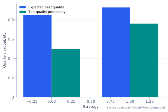
Compare the input regimes
Each case uses invented inputs. The results follow from this model and do not describe measured hardware.
Baseline regime
Complete inputs
- Time budget, seconds
- 80
- Setup per strategy, seconds
- 10
- A seconds per run
- 4
- B seconds per run
- 15
- A high-quality probability
- 0.04
- B high-quality probability
- 0.3
- Quality levels
- 0.4, 0.7, 1
- A fraction of non-top outcomes at lowest quality
- 0.55
- B fraction of non-top outcomes at lowest quality
- 0.3
- Subtract setup before counting complete runs: A fits 17; B fits 4. An unfinished run contributes no result.
- For independent repeats, the probability all answers lie below a quality level is the single-run cumulative probability raised to the number of runs. This gives the distribution of the best answer.
- The top-quality probabilities are 0.500413 and 0.7599. Summing the quality-level increments times their exceedance probabilities gives expected best values 0.850118 and 0.927387.
| Calculated quantity | Synthetic result |
|---|---|
| Completed A runs | 17 |
| Completed B runs | 4 |
| A probability of top-quality answer | 0.5004131923201862 |
| B probability of top-quality answer | 0.7599 |
| A expected best quality | 0.8501181780939879 |
| B expected best quality | 0.927386557 |
| Quality | A probability | B probability |
|---|---|---|
| 0.4 | 0.528 | 0.21 |
| 0.7 | 0.432 | 0.48999999999999994 |
| 1 | 0.04 | 0.3 |
B has the higher expected best quality under the declared deadline. The quality scale, distributions and runtimes are invented. This comparison is meaningful only if both methods solve the same fixed instance and use the same scoring rule; repeated attempts must not silently receive new tuning information.
Comparison regime
Complete inputs
- Time budget, seconds
- 180
- Setup per strategy, seconds
- 20
- A seconds per run
- 6
- B seconds per run
- 20
- A high-quality probability
- 0.07
- B high-quality probability
- 0.4
- Quality levels
- 0.4, 0.7, 1
- A fraction of non-top outcomes at lowest quality
- 0.55
- B fraction of non-top outcomes at lowest quality
- 0.3
- Subtract setup before counting complete runs: A fits 26; B fits 8. An unfinished run contributes no result.
- For independent repeats, the probability all answers lie below a quality level is the single-run cumulative probability raised to the number of runs. This gives the distribution of the best answer.
- The top-quality probabilities are 0.84845 and 0.983204. Summing the quality-level increments times their exceedance probabilities gives expected best values 0.954535 and 0.994961.
| Calculated quantity | Synthetic result |
|---|---|
| Completed A runs | 26 |
| Completed B runs | 8 |
| A probability of top-quality answer | 0.8484497481581527 |
| B probability of top-quality answer | 0.98320384 |
| A expected best quality | 0.9545349163730907 |
| B expected best quality | 0.9949608214011828 |
| Quality | A probability | B probability |
|---|---|---|
| 0.4 | 0.5115 | 0.18 |
| 0.7 | 0.4185 | 0.42 |
| 1 | 0.07 | 0.4 |
B has the higher expected best quality under the declared deadline. The quality scale, distributions and runtimes are invented. This comparison is meaningful only if both methods solve the same fixed instance and use the same scoring rule; repeated attempts must not silently receive new tuning information.
Extended regime
Complete inputs
- Time budget, seconds
- 300
- Setup per strategy, seconds
- 32
- A seconds per run
- 6
- B seconds per run
- 26
- A high-quality probability
- 0.10600000000000001
- B high-quality probability
- 0.52
- Quality levels
- 0.4, 0.7, 1
- A fraction of non-top outcomes at lowest quality
- 0.55
- B fraction of non-top outcomes at lowest quality
- 0.3
- Subtract setup before counting complete runs: A fits 44; B fits 10. An unfinished run contributes no result.
- For independent repeats, the probability all answers lie below a quality level is the single-run cumulative probability raised to the number of runs. This gives the distribution of the best answer.
- The top-quality probabilities are 0.992775 and 0.999351. Summing the quality-level increments times their exceedance probabilities gives expected best values 0.997832 and 0.999805.
| Calculated quantity | Synthetic result |
|---|---|
| Completed A runs | 44 |
| Completed B runs | 10 |
| A probability of top-quality answer | 0.9927747841325296 |
| B probability of top-quality answer | 0.9993507493789145 |
| A expected best quality | 0.9978324352397507 |
| B expected best quality | 0.9998052236635464 |
| Quality | A probability | B probability |
|---|---|---|
| 0.4 | 0.4917 | 0.144 |
| 0.7 | 0.4023 | 0.33599999999999997 |
| 1 | 0.10600000000000001 | 0.52 |
B has the higher expected best quality under the declared deadline. The quality scale, distributions and runtimes are invented. This comparison is meaningful only if both methods solve the same fixed instance and use the same scoring rule; repeated attempts must not silently receive new tuning information.
Try the reasoning: Which strategy maximizes the expected best score, and which maximizes top-quality probability? Would a different deadline change the choice?
Algorithms and useful workThe most likely single quantum search is not always the best campaignHow should an ideal search trade amplification depth for additional attempts?
Amplitude amplification rotates an ideal state toward a marked subspace, but continuing the rotation can move it away again. A familiar teaching problem asks how many iterations maximize the success of one attempt. A complete workflow can ask a different question: how many iterations leave the best overall chance of success within one time budget?
The lab uses the ideal two-dimensional rotation formula and adds an explicit preparation cost and oracle-equivalent timing convention. Each candidate depth allows a different number of complete restarts. The campaign success is then calculated from those independent attempts. The best single attempt and best whole campaign are reported separately rather than forcing them into one headline ratio.
This is an extension of an algorithm lesson, not a practical speedup estimate. A real oracle must be constructed and uncomputed, data preparation must be counted, and marked outputs need verification. Those costs can dominate an application. The useful interaction lets the reader increase preparation cost while leaving the ideal quantum rotation unchanged, making clear that algorithmic probability and complete workload time are separate layers of evidence.
Start with the assumptions
- The ideal amplitude-amplification model is exact in the synthetic calculation.
- The timing convention is chosen for this exercise.
- Restarts are independent and verification is included only through the declared budget convention.
theta = asin(sqrt(marked fraction))
Ideal per-attempt success = sin²((2k+1)theta)
Declared attempt time = preparation + (2k+1) × oracle-equivalent time
Campaign success = 1-(1-per-attempt success)^complete_attempts
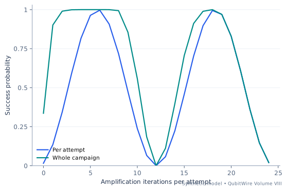
Compare the input regimes
Each case uses invented inputs. The results follow from this model and do not describe measured hardware.
Baseline regime
Complete inputs
- Marked fraction
- 0.015625
- Oracle-equivalent time
- 1
- Preparation time
- 2
- Total time budget
- 80
- Maximum iterations per attempt
- 24
- The ideal success after k iterations is sin²((2k+1)theta), where theta = asin(sqrt(0.015625)).
- The declared attempt time is preparation + (2k+1) × oracle-equivalent time. The factor 2k+1 is this exercise’s accounting convention, not a universal decomposition of a Grover circuit.
- At k = 6, 5 complete independent attempts fit. Their combined success is 1-(1-p)^attempts = 1.
| Calculated quantity | Synthetic result |
|---|---|
| Best tested iterations per attempt | 6 |
| Attempts fitting the budget | 5 |
| Success per chosen attempt | 0.9965856807867991 |
| Campaign success probability | 0.999999999999536 |
| Best single-attempt iteration count | 6 |
| Unamplified campaign success | 0.3359894766227789 |
| Iterations | Single-attempt success | Duration | Complete attempts | Campaign success |
|---|---|---|---|---|
| 0 | 0.015625 | 3 | 26 | 0.3359894766227789 |
| 6 | 0.9965856807867991 | 15 | 5 | 0.999999999999536 |
The best tested campaign choice is k = 6; the best single-attempt probability occurs at k = 6. They optimize different quantities. A real advantage claim must also establish the oracle construction, state preparation, verification and fair classical search cost; this ideal rotation model supplies none of those performance facts.
Comparison regime
Complete inputs
- Marked fraction
- 0.004464285714285714
- Oracle-equivalent time
- 1.5
- Preparation time
- 27
- Total time budget
- 180
- Maximum iterations per attempt
- 24
- The ideal success after k iterations is sin²((2k+1)theta), where theta = asin(sqrt(0.004464)).
- The declared attempt time is preparation + (2k+1) × oracle-equivalent time. The factor 2k+1 is this exercise’s accounting convention, not a universal decomposition of a Grover circuit.
- At k = 11, 2 complete independent attempts fit. Their combined success is 1-(1-p)^attempts = 0.999999.
| Calculated quantity | Synthetic result |
|---|---|
| Best tested iterations per attempt | 11 |
| Attempts fitting the budget | 2 |
| Success per chosen attempt | 0.9989180813519019 |
| Campaign success probability | 0.9999988294520389 |
| Best single-attempt iteration count | 11 |
| Unamplified campaign success | 0.026488540084901542 |
| Iterations | Single-attempt success | Duration | Complete attempts | Campaign success |
|---|---|---|---|---|
| 0 | 0.004464285714285715 | 28.5 | 6 | 0.026488540084901542 |
| 11 | 0.9989180813519019 | 61.5 | 2 | 0.9999988294520389 |
The best tested campaign choice is k = 11; the best single-attempt probability occurs at k = 11. They optimize different quantities. A real advantage claim must also establish the oracle construction, state preparation, verification and fair classical search cost; this ideal rotation model supplies none of those performance facts.
Extended regime
Complete inputs
- Marked fraction
- 0.002403846153846154
- Oracle-equivalent time
- 2.1
- Preparation time
- 57
- Total time budget
- 300
- Maximum iterations per attempt
- 24
- The ideal success after k iterations is sin²((2k+1)theta), where theta = asin(sqrt(0.002404)).
- The declared attempt time is preparation + (2k+1) × oracle-equivalent time. The factor 2k+1 is this exercise’s accounting convention, not a universal decomposition of a Grover circuit.
- At k = 16, 2 complete independent attempts fit. Their combined success is 1-(1-p)^attempts = 0.999995.
| Calculated quantity | Synthetic result |
|---|---|
| Best tested iterations per attempt | 16 |
| Attempts fitting the budget | 2 |
| Success per chosen attempt | 0.9977158771365623 |
| Campaign success probability | 0.9999947827827447 |
| Best single-attempt iteration count | 16 |
| Unamplified campaign success | 0.011961584744724526 |
| Iterations | Single-attempt success | Duration | Complete attempts | Campaign success |
|---|---|---|---|---|
| 0 | 0.002403846153846154 | 59.1 | 5 | 0.011961584744724526 |
| 16 | 0.9977158771365623 | 126.3 | 2 | 0.9999947827827447 |
The best tested campaign choice is k = 16; the best single-attempt probability occurs at k = 16. They optimize different quantities. A real advantage claim must also establish the oracle construction, state preparation, verification and fair classical search cost; this ideal rotation model supplies none of those performance facts.
Try the reasoning: Compare the campaign optimum with the single-attempt optimum. Which preparation and restart costs make their objectives differ?
Sources and model boundaries
- Grover's algorithm ↗
Ideal amplitude amplification rotates a state in a two-dimensional subspace and can overshoot the desired marked population. The lab's timing convention and campaign budget are independently chosen; no hardware runtime, API version or practical advantage is claimed.
Algorithms and useful workA small experiment schedule should expose what it valuesWhich subset of experiments fits the available time under a declared additive objective?
A laboratory may have more worthwhile experiments than available time. The choice is rarely settled by selecting the fastest experiment or the one with the largest individual expected value. Some combinations fit the schedule better than others. The objective also deserves scrutiny: a numerical value assigned to a task is a planning preference until it has a defensible information model behind it.
This example enumerates every subset of eight tasks, keeping only schedules under a fixed time budget. It compares the exact best subset with input-order packing and a value-per-time greedy rule. Because the example is small, exhaustive classical search is transparent and cheap. It demonstrates the optimization problem without creating a claim that quantum computation is required to solve it.
The cases give all task durations and values, along with the exact selected subset. The most useful follow-up is to challenge the assumptions: two experiments may answer the same question, one may enable another, or learning from an early result may change the remaining choices. Those effects require dependencies or adaptive information value. Stating the simple objective makes those omissions easier to discuss than hiding the choice behind a generic intelligent scheduler label.
Start with the assumptions
- Task values are additive, known and invented.
- Task durations are fixed.
- There are no dependencies or benefits from partial completion.
Choose a subset S with sum_{i in S} time_i <= available time
Maximize sum_{i in S} declared learning_value_i
Eight tasks have 2^8 = 256 subsets
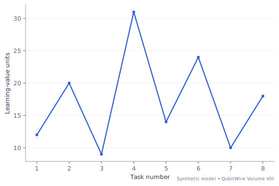
Compare the input regimes
Each case uses invented inputs. The results follow from this model and do not describe measured hardware.
Baseline regime
Complete inputs
- Task durations
- 9, 14, 7, 20, 11, 17, 8, 13
- Declared learning values
- 12, 20, 9, 31, 14, 24, 10, 18
- Available time
- 35
- Enumerate every subset of 8 tasks: 2^8 = 256 candidates. Keep only those whose total time does not exceed 35.
- Maximize the declared value sum, breaking ties by less time. The selected tasks are 2, 4, taking 34 time units.
- Input-order packing gives value 41; greedy value-per-time packing gives 51. The exact search gives 51.
| Calculated quantity | Synthetic result |
|---|---|
| Exact best selected task numbers | 2, 4 |
| Exact best total learning value | 51 |
| Exact best used time | 34 |
| Input-order schedule value | 41 |
| Value-per-time greedy schedule value | 51 |
| Total subsets checked | 256 |
| Task | Duration | Declared learning value | Selected by exact search |
|---|---|---|---|
| 1 | 9 | 12 | No |
| 2 | 14 | 20 | Yes |
| 3 | 7 | 9 | No |
| 4 | 20 | 31 | Yes |
| 5 | 11 | 14 | No |
| 6 | 17 | 24 | No |
| 7 | 8 | 10 | No |
| 8 | 13 | 18 | No |
This small classical calculation makes an experimental planning objective explicit. The learning values are invented preferences, not measured information gain or a ranking of scientific importance. Dependencies between experiments, uncertain duration and complementary results violate the additive model. No quantum optimization advantage is claimed.
Comparison regime
Complete inputs
- Task durations
- 9, 14, 7, 20, 11, 17, 8, 13
- Declared learning values
- 17, 20, 19, 31, 19, 24, 15, 18
- Available time
- 50
- Enumerate every subset of 8 tasks: 2^8 = 256 candidates. Keep only those whose total time does not exceed 50.
- Maximize the declared value sum, breaking ties by less time. The selected tasks are 1, 2, 3, 5, 7, taking 49 time units.
- Input-order packing gives value 87; greedy value-per-time packing gives 90. The exact search gives 90.
| Calculated quantity | Synthetic result |
|---|---|
| Exact best selected task numbers | 1, 2, 3, 5, 7 |
| Exact best total learning value | 90 |
| Exact best used time | 49 |
| Input-order schedule value | 87 |
| Value-per-time greedy schedule value | 90 |
| Total subsets checked | 256 |
| Task | Duration | Declared learning value | Selected by exact search |
|---|---|---|---|
| 1 | 9 | 17 | Yes |
| 2 | 14 | 20 | Yes |
| 3 | 7 | 19 | Yes |
| 4 | 20 | 31 | No |
| 5 | 11 | 19 | Yes |
| 6 | 17 | 24 | No |
| 7 | 8 | 15 | Yes |
| 8 | 13 | 18 | No |
This small classical calculation makes an experimental planning objective explicit. The learning values are invented preferences, not measured information gain or a ranking of scientific importance. Dependencies between experiments, uncertain duration and complementary results violate the additive model. No quantum optimization advantage is claimed.
Extended regime
Complete inputs
- Task durations
- 9, 14, 7, 20, 11, 17, 8, 13
- Declared learning values
- 23, 20, 31, 31, 25, 24, 21, 18
- Available time
- 68
- Enumerate every subset of 8 tasks: 2^8 = 256 candidates. Keep only those whose total time does not exceed 68.
- Maximize the declared value sum, breaking ties by less time. The selected tasks are 1, 3, 4, 5, 7, 8, taking 68 time units.
- Input-order packing gives value 130; greedy value-per-time packing gives 149. The exact search gives 149.
| Calculated quantity | Synthetic result |
|---|---|
| Exact best selected task numbers | 1, 3, 4, 5, 7, 8 |
| Exact best total learning value | 149 |
| Exact best used time | 68 |
| Input-order schedule value | 130 |
| Value-per-time greedy schedule value | 149 |
| Total subsets checked | 256 |
| Task | Duration | Declared learning value | Selected by exact search |
|---|---|---|---|
| 1 | 9 | 23 | Yes |
| 2 | 14 | 20 | No |
| 3 | 7 | 31 | Yes |
| 4 | 20 | 31 | Yes |
| 5 | 11 | 25 | Yes |
| 6 | 17 | 24 | No |
| 7 | 8 | 21 | Yes |
| 8 | 13 | 18 | Yes |
This small classical calculation makes an experimental planning objective explicit. The learning values are invented preferences, not measured information gain or a ranking of scientific importance. Dependencies between experiments, uncertain duration and complementary results violate the additive model. No quantum optimization advantage is claimed.
Try the reasoning: Why can sorting by learning value per time miss the exact subset optimum? Which dependency between experiments would break the additive model?
Algorithms and useful workA cheaper gradient can spend its savings on an omitted directionHow does ignoring coordinates change the error budget for a variational update?
A variational routine may require many expectation-value measurements to estimate a gradient. Measuring only a subset of parameters appears to reduce the work, but the omitted directions can contribute a systematic error to the update. The fair comparison asks how both choices meet the same gradient-error target.
The model uses a standard two-shift estimator where each derivative is half the difference of two independent sample means. Summing the coordinate variances gives an expected squared Euclidean sampling error. A subset estimator receives an additional squared-error contribution from the known synthetic gradient components it omits. If that contribution already exceeds the target, no number of extra shots on the retained coordinates can repair the estimate.
The omitted norm is supplied by construction, which is a major advantage unavailable in most real optimization runs. The lab should therefore accompany a discussion of screening, pilot estimates or structural assumptions used to select parameters. It explains what a claimed measurement saving must preserve, while avoiding the claim that an actual algorithm can discover harmless omissions without paying for information.
Start with the assumptions
- The gate supports the stated parameter-shift rule.
- Shifted measurements and coordinates are independently estimated.
- Omitted-gradient norm is known only in this synthetic example.
Derivative estimate = (mean_plus - mean_minus)/2
Per-coordinate variance with n shots per shift = v/(2n)
Full expected squared gradient error = parameters × v/(2n)
Subset total = omitted squared norm + active_parameters × v/(2n)
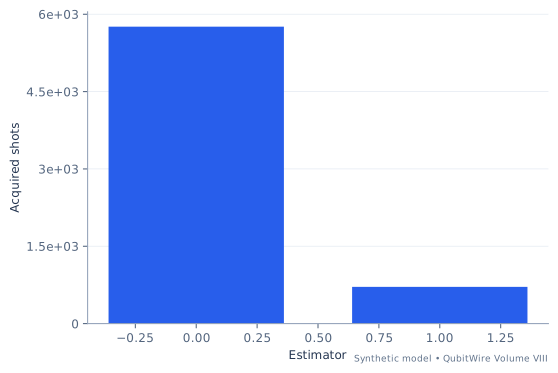
Compare the input regimes
Each case uses invented inputs. The results follow from this model and do not describe measured hardware.
Baseline regime
Complete inputs
- Total parameters
- 12
- Active subset parameters
- 4
- Per-shift shot variance
- 0.4
- Squared gradient-error target
- 0.01
- Squared norm of omitted gradient
- 0.001
- Shot time, milliseconds
- 0.1
- For one parameter, the estimator is (mean_plus - mean_minus)/2. Independent equal-variance shifted samples give variance v/(2n).
- The expected squared Euclidean sampling error sums over 12 coordinates. Set parameters × v/(2n) <= target, giving 240 shots at each of the two shifts.
- The active-subset estimate leaves known synthetic omitted squared norm 0.001. Only 0.009 remains for sampling error; if this is nonpositive, no shot count repairs the omission.
| Calculated quantity | Synthetic result |
|---|---|
| Shots per shift, full gradient | 240 |
| Total full-gradient shots | 5760 |
| Full-gradient acquisition, seconds | 0.576 |
| Subset remaining squared-error budget | 0.009 |
| Total subset-gradient shots | 712 |
| Subset acquisition, seconds | 0.0712 |
Measuring fewer coordinates can reduce work or consume the error budget through omitted directions. The omitted-gradient norm is provided by construction here; an actual optimizer normally does not know it for free. Parameter-shift identities require an appropriate gate generator and shift rule. Correlations within or between the two shifted sample means can change each coordinate variance; cross-coordinate covariance alone does not change the trace-based squared-error sum.
Comparison regime
Complete inputs
- Total parameters
- 22
- Active subset parameters
- 9
- Per-shift shot variance
- 0.4
- Squared gradient-error target
- 0.01
- Squared norm of omitted gradient
- 0.0055
- Shot time, milliseconds
- 0.2
- For one parameter, the estimator is (mean_plus - mean_minus)/2. Independent equal-variance shifted samples give variance v/(2n).
- The expected squared Euclidean sampling error sums over 22 coordinates. Set parameters × v/(2n) <= target, giving 440 shots at each of the two shifts.
- The active-subset estimate leaves known synthetic omitted squared norm 0.0055. Only 0.0045 remains for sampling error; if this is nonpositive, no shot count repairs the omission.
| Calculated quantity | Synthetic result |
|---|---|
| Shots per shift, full gradient | 440 |
| Total full-gradient shots | 19360 |
| Full-gradient acquisition, seconds | 3.872 |
| Subset remaining squared-error budget | 0.0045 |
| Total subset-gradient shots | 7200 |
| Subset acquisition, seconds | 1.44 |
Measuring fewer coordinates can reduce work or consume the error budget through omitted directions. The omitted-gradient norm is provided by construction here; an actual optimizer normally does not know it for free. Parameter-shift identities require an appropriate gate generator and shift rule. Correlations within or between the two shifted sample means can change each coordinate variance; cross-coordinate covariance alone does not change the trace-based squared-error sum.
Extended regime
Complete inputs
- Total parameters
- 34
- Active subset parameters
- 15
- Per-shift shot variance
- 0.4
- Squared gradient-error target
- 0.01
- Squared norm of omitted gradient
- 0.0109
- Shot time, milliseconds
- 0.32
- For one parameter, the estimator is (mean_plus - mean_minus)/2. Independent equal-variance shifted samples give variance v/(2n).
- The expected squared Euclidean sampling error sums over 34 coordinates. Set parameters × v/(2n) <= target, giving 680 shots at each of the two shifts.
- The active-subset estimate leaves known synthetic omitted squared norm 0.0109. Only -0.0009 remains for sampling error; if this is nonpositive, no shot count repairs the omission.
| Calculated quantity | Synthetic result |
|---|---|
| Shots per shift, full gradient | 680 |
| Total full-gradient shots | 46240 |
| Full-gradient acquisition, seconds | 14.796800000000001 |
| Subset remaining squared-error budget | -0.0009 |
| Total subset-gradient shots | Omitted gradient alone exhausts target |
| Subset acquisition, seconds | Infeasible |
Measuring fewer coordinates can reduce work or consume the error budget through omitted directions. The omitted-gradient norm is provided by construction here; an actual optimizer normally does not know it for free. Parameter-shift identities require an appropriate gate generator and shift rule. Correlations within or between the two shifted sample means can change each coordinate variance; cross-coordinate covariance alone does not change the trace-based squared-error sum.
Try the reasoning: When the omitted squared gradient norm meets or exceeds the target, can more shots make the subset estimator feasible?
Sources and model boundaries
- Evaluating analytic gradients on quantum hardware ↗
Parameter-shift identities can estimate exact expectation derivatives for specified gate generators. Finite-sample uncertainty and covariance are independently derived; the two-shift identity is not claimed for every parameterization.
- Combining uncertainty components ↗
Uncertainty propagation includes sensitivities and covariance; independent terms simplify the variance sum. Covariance, bias and distribution assumptions in the teaching models are declared separately; no NIST endorsement is implied.
Sensing and timekeeping
Sensing and timekeepingA longer interrogation can stop being the more informative oneWhat interrogation time best balances phase accumulation, contrast and repeated measurements?
A Ramsey experiment turns a frequency difference into a phase accumulated during a controlled interval. A longer interval makes the phase more sensitive to frequency, but the signal can lose contrast and fewer complete cycles fit into the same campaign. Preparation and readout dead time further change that tradeoff.
This lab uses a local projection-noise expression with independent atoms and a stipulated exponential visibility loss. It counts whole cycles before evaluating the uncertainty. The best point is selected on a declared finite grid, so the answer is a tested numerical minimum rather than an unsupported analytic optimum. Increasing the dead time can change the preferred interrogation even if the atom and contrast law remain identical.
The model does not describe all clock noise. Local oscillator fluctuations, phase wrapping, correlations and systematic shifts can dominate a real experiment. It also predicts a local frequency-estimation uncertainty, not accuracy against a reference. The useful article extension is to place the complete cycle beside the free-evolution interval and show which assumptions allow the stated square-root averaging benefit.
Start with the assumptions
- The experiment operates near the most sensitive fringe point.
- Atoms and complete cycles are independent.
- The exponential contrast law and all time values are invented.
Cycles = floor(campaign/(interrogation + dead time))
C(t) = initial contrast × exp(-t/T2)
Local frequency uncertainty = 1/[2 pi C(t) t sqrt(cycles × atoms)]
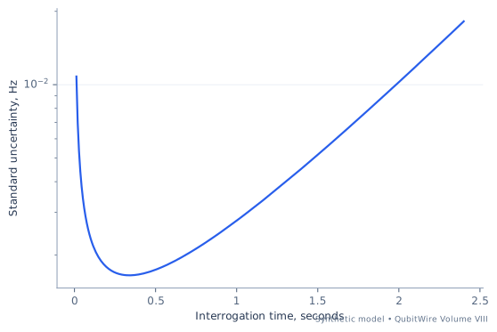
Compare the input regimes
Each case uses invented inputs. The results follow from this model and do not describe measured hardware.
Baseline regime
Complete inputs
- Campaign duration, seconds
- 1200
- Dead time per cycle, seconds
- 0.05
- Visibility decay time, seconds
- 0.6
- Independent atoms per shot
- 100
- Initial contrast
- 0.9
- Interrogation grid points
- 300
- Minimum interrogation / decay time
- 0.02
- Maximum interrogation / decay time
- 4
- Test 300 interrogation times from T2/50 to 4 T2. At each time, floor campaign/(interrogation + dead time) to count complete cycles.
- Use contrast C(t) = initial contrast × exp(-t/T2). At the selected time 0.339452, C = 0.511139 and 3081 cycles fit.
- Near the most sensitive Ramsey fringe point, the stipulated independent projection-noise model gives frequency uncertainty 1/(2 pi C t sqrt(cycles × atoms)) = 0.001653 Hz.
| Calculated quantity | Synthetic result |
|---|---|
| Best tested interrogation, seconds | 0.3394515050167224 |
| Completed cycles | 3081 |
| Visibility at chosen interrogation | 0.5111393506892022 |
| Linearized frequency standard uncertainty, Hz | 0.0016525599638816018 |
| At-T2 reference uncertainty, Hz | 0.0018646829739183317 |
| Best / at-T2 standard uncertainty | 0.8862417831858102 |
Long interrogation increases phase accumulation while reducing visibility and the number of cycles. Dead time changes the balance. The grid optimum is a result of the declared local linear-response model; oscillator noise, phase wrapping, correlations and systematic shifts are excluded. It is not a measured clock accuracy or a universal optimum.
Comparison regime
Complete inputs
- Campaign duration, seconds
- 1200
- Dead time per cycle, seconds
- 0.55
- Visibility decay time, seconds
- 1.2
- Independent atoms per shot
- 350
- Initial contrast
- 0.85
- Interrogation grid points
- 300
- Minimum interrogation / decay time
- 0.02
- Maximum interrogation / decay time
- 4
- Test 300 interrogation times from T2/50 to 4 T2. At each time, floor campaign/(interrogation + dead time) to count complete cycles.
- Use contrast C(t) = initial contrast × exp(-t/T2). At the selected time 0.838635, C = 0.422578 and 864 cycles fit.
- Near the most sensitive Ramsey fringe point, the stipulated independent projection-noise model gives frequency uncertainty 1/(2 pi C t sqrt(cycles × atoms)) = 0.000817 Hz.
| Calculated quantity | Synthetic result |
|---|---|
| Best tested interrogation, seconds | 0.8386354515050167 |
| Completed cycles | 864 |
| Visibility at chosen interrogation | 0.42257775832249656 |
| Linearized frequency standard uncertainty, Hz | 0.0008166752346075334 |
| At-T2 reference uncertainty, Hz | 0.0008662338163331558 |
| Best / at-T2 standard uncertainty | 0.9427884471938439 |
Long interrogation increases phase accumulation while reducing visibility and the number of cycles. Dead time changes the balance. The grid optimum is a result of the declared local linear-response model; oscillator noise, phase wrapping, correlations and systematic shifts are excluded. It is not a measured clock accuracy or a universal optimum.
Extended regime
Complete inputs
- Campaign duration, seconds
- 1200
- Dead time per cycle, seconds
- 1.1500000000000001
- Visibility decay time, seconds
- 1.92
- Independent atoms per shot
- 650
- Initial contrast
- 0.79
- Interrogation grid points
- 300
- Minimum interrogation / decay time
- 0.02
- Maximum interrogation / decay time
- 4
- Test 300 interrogation times from T2/50 to 4 T2. At each time, floor campaign/(interrogation + dead time) to count complete cycles.
- Use contrast C(t) = initial contrast × exp(-t/T2). At the selected time 1.418488, C = 0.377374 and 467 cycles fit.
- Near the most sensitive Ramsey fringe point, the stipulated independent projection-noise model gives frequency uncertainty 1/(2 pi C t sqrt(cycles × atoms)) = 0.00054 Hz.
| Calculated quantity | Synthetic result |
|---|---|
| Best tested interrogation, seconds | 1.4184882943143813 |
| Completed cycles | 467 |
| Visibility at chosen interrogation | 0.37737408328628846 |
| Linearized frequency standard uncertainty, Hz | 0.0005396437924807968 |
| At-T2 reference uncertainty, Hz | 0.0005664966052937949 |
| Best / at-T2 standard uncertainty | 0.952598457674655 |
Long interrogation increases phase accumulation while reducing visibility and the number of cycles. Dead time changes the balance. The grid optimum is a result of the declared local linear-response model; oscillator noise, phase wrapping, correlations and systematic shifts are excluded. It is not a measured clock accuracy or a universal optimum.
Try the reasoning: Why can a longer interrogation lower local phase noise yet worsen the frequency estimate once visibility and completed cycles are counted?
Sources and model boundaries
- Quantum Limits to Spectroscopy ↗
Independent-atom Ramsey spectroscopy has a projection-noise sensitivity that depends on interrogation time and the number of atoms and measurements. The checked primary excerpt supports the projection-noise relation. The added exponential contrast model, dead time and integer schedule are original synthetic assumptions. Uncertainty is not accuracy.
Sensing and timekeepingCommon noise cancels only when the channels agree on gainHow can a quiet differential measurement still report a false spatial gradient?
Differential sensing compares nearby measurements to reject a disturbance shared by both. That rejection depends on the two channels responding consistently. If one channel amplifies the common signal slightly more than the other, subtracting them can leave a residual that looks like the spatial difference the instrument was meant to measure.
The constructed model places two sensors symmetrically across a constant gradient and assigns one a gain error. The mean inferred gradient can then be expanded into the true gradient, a common-field leakage term and a smaller gradient-proportional gain term. Correlated random noise is propagated separately. The final root mean squared error combines the random spread with the systematic offset instead of treating a quiet trace as an accurate result.
Increasing the separation reduces the conversion of some noise and leakage terms into gradient units. It also changes the region being sampled, so a real field may no longer have a constant gradient across that baseline. A gain comparison therefore needs explicit field and geometry assumptions. This keeps a cancellation mechanism understandable without suggesting that correlation alone eliminates every practical disturbance.
Start with the assumptions
- The true gradient is constant across the separation.
- Only sensor A has the declared gain error.
- Readout noise covariance is known and independent of the mean-field model.
True local fields = B ± G L/2
Estimated gradient = [(1+g)(B+G L/2)-(B-G L/2)]/L
Bias = gB/L + gG/2
Random gradient variance = (s_A²+s_B²-2rho s_A s_B)/L²
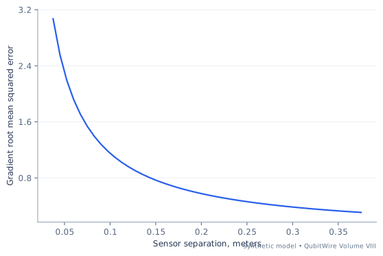
Compare the input regimes
Each case uses invented inputs. The results follow from this model and do not describe measured hardware.
Baseline regime
Complete inputs
- Sensor separation, meters
- 0.15
- True gradient, field units per meter
- 0.6
- Common field, field units
- 40
- A relative gain error
- 0.0002
- A noise standard deviation
- 0.08
- B noise standard deviation
- 0.1
- Noise correlation
- 0.2
- The true sensor fields are B ± G L/2. Multiply A by (1 + gain error), subtract B’s reading, then divide by separation.
- The resulting bias is gB/L + gG/2 = 0.053393. The common field cancels only when the gains match.
- Random variance of the difference is s_A² + s_B² - 2 rho s_A s_B. Dividing its square root by L gives 0.765942, and combining variance with squared bias gives RMSE 0.7678.
| Calculated quantity | Synthetic result |
|---|---|
| Mean inferred gradient | 0.6533933333333646 |
| Gradient bias from gain mismatch | 0.0533933333333646 |
| Gradient random standard uncertainty | 0.7659416862050705 |
| Gradient root mean squared error | 0.7678004393793445 |
| Shared-field leakage term gB/L | 0.05333333333333334 |
| Gradient-proportional gain term gG/2 | 0.00006 |
The common-field leakage contributes 0.053333 gradient units. A quiet difference can still be biased if gain mismatch converts a large shared field into an apparent gradient. Increasing separation changes both noise conversion and spatial interpretation; the model assumes a constant gradient across every tested baseline.
Comparison regime
Complete inputs
- Sensor separation, meters
- 0.35
- True gradient, field units per meter
- 0.6
- Common field, field units
- 65
- A relative gain error
- 0.0012000000000000001
- A noise standard deviation
- 0.08
- B noise standard deviation
- 0.1
- Noise correlation
- 0.45
- The true sensor fields are B ± G L/2. Multiply A by (1 + gain error), subtract B’s reading, then divide by separation.
- The resulting bias is gB/L + gG/2 = 0.223217. The common field cancels only when the gains match.
- Random variance of the difference is s_A² + s_B² - 2 rho s_A s_B. Dividing its square root by L gives 0.274048, and combining variance with squared bias gives RMSE 0.353451.
| Calculated quantity | Synthetic result |
|---|---|
| Mean inferred gradient | 0.823217142857199 |
| Gradient bias from gain mismatch | 0.22321714285719907 |
| Gradient random standard uncertainty | 0.27404751561786966 |
| Gradient root mean squared error | 0.3534514587346581 |
| Shared-field leakage term gB/L | 0.22285714285714292 |
| Gradient-proportional gain term gG/2 | 0.00036 |
The common-field leakage contributes 0.222857 gradient units. A quiet difference can still be biased if gain mismatch converts a large shared field into an apparent gradient. Increasing separation changes both noise conversion and spatial interpretation; the model assumes a constant gradient across every tested baseline.
Extended regime
Complete inputs
- Sensor separation, meters
- 0.59
- True gradient, field units per meter
- 0.6
- Common field, field units
- 95
- A relative gain error
- 0.0024000000000000002
- A noise standard deviation
- 0.08
- B noise standard deviation
- 0.1
- Noise correlation
- 0.75
- The true sensor fields are B ± G L/2. Multiply A by (1 + gain error), subtract B’s reading, then divide by separation.
- The resulting bias is gB/L + gG/2 = 0.387161. The common field cancels only when the gains match.
- Random variance of the difference is s_A² + s_B² - 2 rho s_A s_B. Dividing its square root by L gives 0.112428, and combining variance with squared bias gives RMSE 0.403154.
| Calculated quantity | Synthetic result |
|---|---|
| Mean inferred gradient | 0.987160677966123 |
| Gradient bias from gain mismatch | 0.38716067796612297 |
| Gradient random standard uncertainty | 0.11242795899509833 |
| Gradient root mean squared error | 0.4031543581892567 |
| Shared-field leakage term gB/L | 0.3864406779661017 |
| Gradient-proportional gain term gG/2 | 0.00072 |
The common-field leakage contributes 0.386441 gradient units. A quiet difference can still be biased if gain mismatch converts a large shared field into an apparent gradient. Increasing separation changes both noise conversion and spatial interpretation; the model assumes a constant gradient across every tested baseline.
Try the reasoning: Compare the common-field leakage gB/L with the true gradient. Can a small random standard uncertainty certify the measurement as accurate?
Sources and model boundaries
- Combining uncertainty components ↗
Uncertainty propagation includes sensitivities and covariance; independent terms simplify the variance sum. Covariance, bias and distribution assumptions in the teaching models are declared separately; no NIST endorsement is implied.
Sensing and timekeepingThree clock comparisons can reveal an inconsistent linkWhat can a closed comparison loop establish without an absolute time reference?
A pairwise clock comparison reports a relative offset. With three clocks and three pairwise measurements, the numbers should close around the loop if they represent consistent offsets at the same time. Adding B minus A to C minus B should reproduce C minus A. A nonzero closure signals inconsistency in the comparison set.
The lab first calculates that closure and its uncertainty under independent edge errors. It then fixes clock A as an arbitrary zero and fits the two remaining offsets by weighted least squares. The fitted comparisons close exactly, while residuals show how the original observations depart from one consistent set of clock values. The weights express the relative uncertainties assigned to the links.
A failed closure cannot, by itself, identify which clock or transfer path is responsible. A common offset shared by every clock can also escape the loop entirely. These limits make the example useful for an article about networked clocks or time transfer: internal consistency and accuracy against an external reference are different achievements. The coordinate choice A equals zero is bookkeeping, not a claim that A is the truth.
Start with the assumptions
- Comparisons refer to one common epoch.
- Edge errors are independent with known standard uncertainties.
- Clock A is fixed to zero only to choose a reference coordinate.
Loop closure = measured(B-A) + measured(C-B) - measured(C-A)
Independent closure uncertainty = sqrt(s_AB²+s_BC²+s_AC²)
Weighted least-squares offsets solve (X^T W X) beta = X^T W y
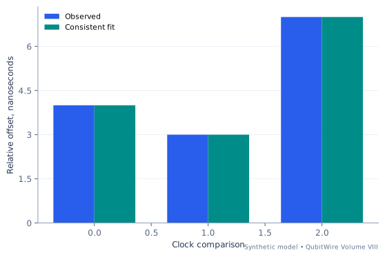
Compare the input regimes
Each case uses invented inputs. The results follow from this model and do not describe measured hardware.
Baseline regime
Complete inputs
- Measured B minus A, nanoseconds
- 4
- Measured C minus B, nanoseconds
- 3
- Measured C minus A, nanoseconds
- 7
- Edge standard uncertainties, nanoseconds
- 0.4, 0.7, 0.5
- If all comparisons reflected consistent offsets, (B-A) + (C-B) - (C-A) would equal zero. The observed closure is 0 nanoseconds.
- With independent edge errors, closure uncertainty is sqrt(s_AB²+s_BC²+s_AC²) = 0.948683. The standardized closure is 0.
- Fix clock A as the arbitrary zero and solve weighted least squares for B and C. The fitted offsets are 4 and 7; residuals are 0, -8.88178e-16, -8.88178e-16.
| Calculated quantity | Synthetic result |
|---|---|
| Observed loop closure, nanoseconds | 0 |
| Loop standard uncertainty, nanoseconds | 0.9486832980505138 |
| Closure / standard uncertainty | 0 |
| Fitted B offset relative to A, nanoseconds | 4 |
| Fitted C offset relative to A, nanoseconds | 7.000000000000001 |
| Weighted residual sum of squares | 4.765363835620806e-30 |
| Comparison | Observed, ns | Standard uncertainty, ns | Residual, ns |
|---|---|---|---|
| B − A | 4 | 0.4 | 0 |
| C − B | 3 | 0.7 | -8.881784197001252e-16 |
| C − A | 7 | 0.5 | -8.881784197001252e-16 |
The loop detects inconsistent comparisons but cannot identify the responsible clock or link by itself. A shared calibration offset can evade the loop entirely, and correlated transfer errors change its uncertainty. Fixing A to zero is a coordinate choice, not evidence that clock A is accurate against an external time standard.
Comparison regime
Complete inputs
- Measured B minus A, nanoseconds
- 5
- Measured C minus B, nanoseconds
- 2.5
- Measured C minus A, nanoseconds
- 9
- Edge standard uncertainties, nanoseconds
- 0.5, 0.7, 0.5
- If all comparisons reflected consistent offsets, (B-A) + (C-B) - (C-A) would equal zero. The observed closure is -1.5 nanoseconds.
- With independent edge errors, closure uncertainty is sqrt(s_AB²+s_BC²+s_AC²) = 0.994987. The standardized closure is -1.507557.
- Fix clock A as the arbitrary zero and solve weighted least squares for B and C. The fitted offsets are 5.378788 and 8.621212; residuals are -0.378788, -0.742424, 0.378788.
| Calculated quantity | Synthetic result |
|---|---|
| Observed loop closure, nanoseconds | -1.5 |
| Loop standard uncertainty, nanoseconds | 0.99498743710662 |
| Closure / standard uncertainty | -1.507556722888818 |
| Fitted B offset relative to A, nanoseconds | 5.378787878787879 |
| Fitted C offset relative to A, nanoseconds | 8.621212121212123 |
| Weighted residual sum of squares | 2.272727272727273 |
| Comparison | Observed, ns | Standard uncertainty, ns | Residual, ns |
|---|---|---|---|
| B − A | 5 | 0.5 | -0.3787878787878789 |
| C − B | 2.5 | 0.7 | -0.742424242424244 |
| C − A | 9 | 0.5 | 0.3787878787878771 |
The loop detects inconsistent comparisons but cannot identify the responsible clock or link by itself. A shared calibration offset can evade the loop entirely, and correlated transfer errors change its uncertainty. Fixing A to zero is a coordinate choice, not evidence that clock A is accurate against an external time standard.
Extended regime
Complete inputs
- Measured B minus A, nanoseconds
- 6.2
- Measured C minus B, nanoseconds
- 1.9
- Measured C minus A, nanoseconds
- 11.4
- Edge standard uncertainties, nanoseconds
- 0.62, 0.7, 0.5
- If all comparisons reflected consistent offsets, (B-A) + (C-B) - (C-A) would equal zero. The observed closure is -3.3 nanoseconds.
- With independent edge errors, closure uncertainty is sqrt(s_AB²+s_BC²+s_AC²) = 1.060377. The standardized closure is -3.1121.
- Fix clock A as the arbitrary zero and solve weighted least squares for B and C. The fitted offsets are 7.328175 and 10.666275; residuals are -1.128175, -1.4381, 0.733725.
| Calculated quantity | Synthetic result |
|---|---|
| Observed loop closure, nanoseconds | -3.3000000000000007 |
| Loop standard uncertainty, nanoseconds | 1.060377291344925 |
| Closure / standard uncertainty | -3.112099841193751 |
| Fitted B offset relative to A, nanoseconds | 7.3281750266808965 |
| Fitted C offset relative to A, nanoseconds | 10.666275346851654 |
| Weighted residual sum of squares | 9.685165421558166 |
| Comparison | Observed, ns | Standard uncertainty, ns | Residual, ns |
|---|---|---|---|
| B − A | 6.2 | 0.62 | -1.1281750266808963 |
| C − B | 1.9 | 0.7 | -1.4381003201707574 |
| C − A | 11.4 | 0.5 | 0.7337246531483466 |
The loop detects inconsistent comparisons but cannot identify the responsible clock or link by itself. A shared calibration offset can evade the loop entirely, and correlated transfer errors change its uncertainty. Fixing A to zero is a coordinate choice, not evidence that clock A is accurate against an external time standard.
Try the reasoning: Would a shared offset in all clocks be visible in the loop closure? Explain what setting clock A to zero actually fixes.
Sources and model boundaries
- Combining uncertainty components ↗
Uncertainty propagation includes sensitivities and covariance; independent terms simplify the variance sum. Covariance, bias and distribution assumptions in the teaching models are declared separately; no NIST endorsement is implied.
Sensing and timekeepingA stability curve remembers how the data were madeHow does a known drift appear when adjacent averages are compared?
A time series can look quieter after averaging while still changing systematically from one interval to the next. Frequency-stability analysis therefore often compares adjacent averages rather than treating all observations as unrelated draws around a fixed mean. The chosen averaging time becomes part of the question.
This lab constructs a finite record from a repeated bounded pattern plus a linear drift. For several averaging factors, it forms non-overlapping block means and calculates half the mean squared difference between adjacent blocks. The square root is the displayed Allan deviation. The corresponding drift-only curve can be derived exactly, making the growth with averaging time easy to interpret.
The periodic pattern is disclosed because it creates its own apparent sweet spots. The minimum of this finite synthetic curve is not a statistically validated optimum for a random clock. A real analysis needs a noise model, data-quality checks, uncertainty estimates and a reason to choose overlapping or non-overlapping estimators. Inspecting the supplied record construction alongside the stability curve reveals where its apparent improvements come from.
Start with the assumptions
- The finite 240-point record is deterministic and fully specified by the supplied pattern, repeat count and drift.
- Non-overlapping adjacent block means are used.
- No white-noise or population confidence claim is attached to the repeated pattern.
Block mean at factor m = mean of m consecutive frequency samples
Non-overlapping Allan variance = one half × mean of adjacent block-mean differences squared
For pure linear drift per sample r, Allan deviation = |r|m/sqrt(2)
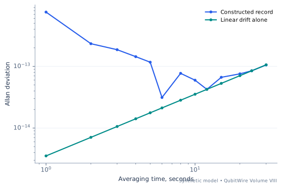
Compare the input regimes
Each case uses invented inputs. The results follow from this model and do not describe measured hardware.
Baseline regime
Complete inputs
- Sampling interval, seconds
- 1
- Drift per sample
- 5e-15
- Bounded fluctuation scale
- 1e-12
- Repeated bounded pattern
- -0.8, 0.5, -0.3, 1, -0.6, 0.2, -1, 0.7, 0.1, -0.2, 0.6, -0.4
- Pattern repeats
- 20
- Tested averaging factors
- 1, 2, 3, 4, 5, 6, 8, 10, 12, 15, 20, 24, 30
- Generate 240 samples from a declared 12-point bounded pattern repeated twenty times, plus linear drift 5e-15 per sample. This is deterministic, not simulated white noise.
- For each averaging factor m, form non-overlapping adjacent block means. Allan variance is one half of the mean squared difference between successive block means.
- The smallest tested deviation is 3.13036e-14 at m = 6, or 6 seconds. Pure linear drift would contribute deviation |slope|m/sqrt(2) = 2.12132e-14.
| Calculated quantity | Synthetic result |
|---|---|
| Smallest deviation among tested averaging factors | 3.130358653436584e-14 |
| Averaging factor at that minimum | 6 |
| Corresponding averaging time, seconds | 6 |
| One-sample Allan deviation | 7.596657145797418e-13 |
| Drift-only deviation at selected factor | 2.1213203435596423e-14 |
| Original frequency samples | 240 |
| Averaging factor | Averaging time, seconds | Non-overlapping Allan deviation |
|---|---|---|
| 1 | 1 | 7.596657145797418e-13 |
| 2 | 2 | 2.3330291918628097e-13 |
| 3 | 3 | 1.8648796260591664e-13 |
| 4 | 4 | 1.437976155479921e-13 |
| 5 | 5 | 1.16954937676049e-13 |
| 6 | 6 | 3.130358653436584e-14 |
| 8 | 8 | 7.713833856042058e-14 |
| 10 | 10 | 5.970944139166223e-14 |
| 12 | 12 | 4.2426406871192846e-14 |
| 15 | 15 | 6.654920207107143e-14 |
| 20 | 20 | 7.573128331625758e-14 |
| 24 | 24 | 8.485281374238569e-14 |
| 30 | 30 | 1.054958059799776e-13 |
The minimum depends on the synthetic periodic pattern as well as drift. It is not a confidence-calibrated estimate of an optimal averaging time for a random clock. The exercise teaches the adjacent-average calculation and shows why a finite stability curve needs a documented data-generating process and sufficient independent information.
Comparison regime
Complete inputs
- Sampling interval, seconds
- 3
- Drift per sample
- 1.5e-14
- Bounded fluctuation scale
- 1.75e-12
- Repeated bounded pattern
- -0.8, 0.5, -0.3, 1, -0.6, 0.2, -1, 0.7, 0.1, -0.2, 0.6, -0.4
- Pattern repeats
- 20
- Tested averaging factors
- 1, 2, 3, 4, 5, 6, 8, 10, 12, 15, 20, 24, 30
- Generate 240 samples from a declared 12-point bounded pattern repeated twenty times, plus linear drift 1.5e-14 per sample. This is deterministic, not simulated white noise.
- For each averaging factor m, form non-overlapping adjacent block means. Allan variance is one half of the mean squared difference between successive block means.
- The smallest tested deviation is 7.49451e-14 at m = 6, or 18 seconds. Pure linear drift would contribute deviation |slope|m/sqrt(2) = 6.36396e-14.
| Calculated quantity | Synthetic result |
|---|---|
| Smallest deviation among tested averaging factors | 7.494513662855988e-14 |
| Averaging factor at that minimum | 6 |
| Corresponding averaging time, seconds | 18 |
| One-sample Allan deviation | 1.3294497988951771e-12 |
| Drift-only deviation at selected factor | 6.363961030678927e-14 |
| Original frequency samples | 240 |
| Averaging factor | Averaging time, seconds | Non-overlapping Allan deviation |
|---|---|---|
| 1 | 3 | 1.3294497988951771e-12 |
| 2 | 6 | 4.086997405690106e-13 |
| 3 | 9 | 3.2750256330794895e-13 |
| 4 | 12 | 2.538848320497214e-13 |
| 5 | 15 | 2.0971041330083852e-13 |
| 6 | 18 | 7.494513662855988e-14 |
| 8 | 24 | 1.511943070376773e-13 |
| 10 | 30 | 1.363015957353398e-13 |
| 12 | 36 | 1.2727922061357854e-13 |
| 15 | 45 | 1.7521389045223385e-13 |
| 20 | 60 | 2.1668718944178915e-13 |
| 24 | 72 | 2.5455844122715713e-13 |
| 30 | 90 | 3.171246687906123e-13 |
The minimum depends on the synthetic periodic pattern as well as drift. It is not a confidence-calibrated estimate of an optimal averaging time for a random clock. The exercise teaches the adjacent-average calculation and shows why a finite stability curve needs a documented data-generating process and sufficient independent information.
Extended regime
Complete inputs
- Sampling interval, seconds
- 3
- Drift per sample
- 2.7e-14
- Bounded fluctuation scale
- 2.65e-12
- Repeated bounded pattern
- -0.8, 0.5, -0.3, 1, -0.6, 0.2, -1, 0.7, 0.1, -0.2, 0.6, -0.4
- Pattern repeats
- 20
- Tested averaging factors
- 1, 2, 3, 4, 5, 6, 8, 10, 12, 15, 20, 24, 30
- Generate 240 samples from a declared 12-point bounded pattern repeated twenty times, plus linear drift 2.7e-14 per sample. This is deterministic, not simulated white noise.
- For each averaging factor m, form non-overlapping adjacent block means. Allan variance is one half of the mean squared difference between successive block means.
- The smallest tested deviation is 1.2906e-13 at m = 6, or 18 seconds. Pure linear drift would contribute deviation |slope|m/sqrt(2) = 1.14551e-13.
| Calculated quantity | Synthetic result |
|---|---|
| Smallest deviation among tested averaging factors | 1.290599310861656e-13 |
| Averaging factor at that minimum | 6 |
| Corresponding averaging time, seconds | 18 |
| One-sample Allan deviation | 2.0131980174146246e-12 |
| Drift-only deviation at selected factor | 1.145512985522207e-13 |
| Original frequency samples | 240 |
| Averaging factor | Averaging time, seconds | Non-overlapping Allan deviation |
|---|---|---|
| 1 | 3 | 2.0131980174146246e-12 |
| 2 | 6 | 6.192708770139663e-13 |
| 3 | 9 | 4.969849396501868e-13 |
| 4 | 12 | 3.865899037838768e-13 |
| 5 | 15 | 3.221027819309538e-13 |
| 6 | 18 | 1.290599310861656e-13 |
| 8 | 24 | 2.4314441295158097e-13 |
| 10 | 30 | 2.313022561404279e-13 |
| 12 | 36 | 2.2910259710444143e-13 |
| 15 | 45 | 3.079292787974874e-13 |
| 20 | 60 | 3.8725880690144055e-13 |
| 24 | 72 | 4.582051942088829e-13 |
| 30 | 90 | 5.711057431345528e-13 |
The minimum depends on the synthetic periodic pattern as well as drift. It is not a confidence-calibrated estimate of an optimal averaging time for a random clock. The exercise teaches the adjacent-average calculation and shows why a finite stability curve needs a documented data-generating process and sufficient independent information.
Try the reasoning: Which averaging factors align with the constructed twelve-sample pattern? Why does the resulting minimum not estimate a random-clock confidence bound?
Sources and model boundaries
- Handbook of Frequency Stability Analysis, NIST SP 1065 ↗
Frequency stability can be characterized through differences between averages at stated averaging times; estimator choice and noise processes matter. The supplied sequence is deterministic and periodic with an added drift. Its calculated minimum is not a population confidence result.