
What changes when two implementations experience the same batch disturbance?
When A and B share an experimental batch, their within-batch difference can remove a common disturbance. The uncertainty then comes from the variation between those differences.
Source research checked . Teaching calculations are ideal models.
Imagine comparing two pulse implementations during a day when a laboratory drifts between warmer and cooler operating conditions. Running all of A first and all of B later confounds implementation with time. Even if the total number of shots is large, a difference between the batches can masquerade as a difference between the methods. The experimental unit must be identified before the error bar is chosen.
A matched design asks A and B to encounter similar conditions and records their difference within each match. A disturbance shared by both measurements can then cancel. The relevant variation is the variation of the differences, rather than the sum of two variances treated as unrelated. Pairing earns this benefit only when the correspondence is real. Pairing unrelated records after inspecting their outcomes is not the same experiment.
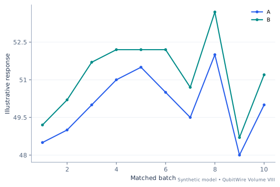
This laboratory constructs ten matched batches with a shared disturbance and smaller difference noise. Its calculation shows the exact standard-error consequence of retaining or discarding the match. The learning goal is to ask what was randomized, what was repeated, and which conditions were shared. A quantum benchmark can have thousands of circuit shots while still having very few independent calibration batches.
Start with the assumptions
- Each pair shares the declared disturbance.
- Difference-noise values are constructed, not sampled from a fitted distribution.
- The sample standard deviation uses denominator n - 1.
d_i = B_i - A_i; mean difference = sum(d_i)/n
SE_paired = sample_SD(d)/sqrt(n)
SE_unpaired = sqrt(sample_Var(A)/n + sample_Var(B)/n)
Compare the input regimes
Each case uses invented inputs. The results follow from this model and do not describe measured hardware.
Baseline regime
Complete inputs
- Common disturbance scale
- 0.5
- Difference noise scale
- 0.5
- True shift
- 1.2
- Response baseline
- 50
- Shared disturbance pattern
- -3, -2, 0, 2, 3, 1, -1, 4, -4, 0
- Difference-noise pattern
- -1, 0, 1, 0, -1, 1, 0, 1, -1, 0
- Compute ten matched differences B_i - A_i. Their mean is 1.2 and their sample standard deviation is 0.408248.
- Divide the difference standard deviation by sqrt(10), giving 0.129099. Treating the same observations as unpaired gives 0.632456.
- The paired calculation retains the shared disturbance as covariance; it cancels in each difference. The unpaired expression discards that relationship.
| Calculated quantity | Synthetic result |
|---|---|
| Batch pairs | 10 |
| Mean B minus A | 1.2 |
| Paired standard error | 0.129099444874 |
| Unpaired standard error | 0.632455532034 |
| Unpaired / paired variance | 24 |
| Pair | A | B | B − A |
|---|---|---|---|
| 1 | 48.5 | 49.2 | 0.7 |
| 2 | 49 | 50.2 | 1.2 |
| 3 | 50 | 51.7 | 1.7 |
| 4 | 51 | 52.2 | 1.2 |
| 5 | 51.5 | 52.2 | 0.7 |
| 6 | 50.5 | 52.2 | 1.7 |
| 7 | 49.5 | 50.7 | 1.2 |
| 8 | 52 | 53.7 | 1.7 |
| 9 | 48 | 48.7 | 0.7 |
| 10 | 50 | 51.2 | 1.2 |
The variance ratio is 24 in this constructed batch. Matching is useful because the common disturbance is genuinely shared. These ten deliberately chosen observations do not validate a population distribution or establish a significance level.
Comparison regime
Complete inputs
- Common disturbance scale
- 2
- Difference noise scale
- 0.62
- True shift
- 1.95
- Response baseline
- 50
- Shared disturbance pattern
- -3, -2, 0, 2, 3, 1, -1, 4, -4, 0
- Difference-noise pattern
- -1, 0, 1, 0, -1, 1, 0, 1, -1, 0
- Compute ten matched differences B_i - A_i. Their mean is 1.95 and their sample standard deviation is 0.506228.
- Divide the difference standard deviation by sqrt(10), giving 0.160083. Treating the same observations as unpaired gives 2.367902.
- The paired calculation retains the shared disturbance as covariance; it cancels in each difference. The unpaired expression discards that relationship.
| Calculated quantity | Synthetic result |
|---|---|
| Batch pairs | 10 |
| Mean B minus A | 1.95 |
| Paired standard error | 0.160083311643 |
| Unpaired standard error | 2.367902025 |
| Unpaired / paired variance | 218.79396462 |
| Pair | A | B | B − A |
|---|---|---|---|
| 1 | 44 | 45.33 | 1.33 |
| 2 | 46 | 47.95 | 1.95 |
| 3 | 50 | 52.57 | 2.57 |
| 4 | 54 | 55.95 | 1.95 |
| 5 | 56 | 57.33 | 1.33 |
| 6 | 52 | 54.57 | 2.57 |
| 7 | 48 | 49.95 | 1.95 |
| 8 | 58 | 60.57 | 2.57 |
| 9 | 42 | 43.33 | 1.33 |
| 10 | 50 | 51.95 | 1.95 |
The variance ratio is 218.793965 in this constructed batch. Matching is useful because the common disturbance is genuinely shared. These ten deliberately chosen observations do not validate a population distribution or establish a significance level.
Extended regime
Complete inputs
- Common disturbance scale
- 3.8
- Difference noise scale
- 0.86
- True shift
- 2.8499999999999996
- Response baseline
- 50
- Shared disturbance pattern
- -3, -2, 0, 2, 3, 1, -1, 4, -4, 0
- Difference-noise pattern
- -1, 0, 1, 0, -1, 1, 0, 1, -1, 0
- Compute ten matched differences B_i - A_i. Their mean is 2.85 and their sample standard deviation is 0.702187.
- Divide the difference standard deviation by sqrt(10), giving 0.222051. Treating the same observations as unpaired gives 4.467241.
- The paired calculation retains the shared disturbance as covariance; it cancels in each difference. The unpaired expression discards that relationship.
| Calculated quantity | Synthetic result |
|---|---|
| Batch pairs | 10 |
| Mean B minus A | 2.85 |
| Paired standard error | 0.222051045183 |
| Unpaired standard error | 4.46724075913 |
| Unpaired / paired variance | 404.737155219 |
| Pair | A | B | B − A |
|---|---|---|---|
| 1 | 38.6 | 40.59 | 1.99 |
| 2 | 42.4 | 45.25 | 2.85 |
| 3 | 50 | 53.71 | 3.71 |
| 4 | 57.6 | 60.45 | 2.85 |
| 5 | 61.4 | 63.39 | 1.99 |
| 6 | 53.8 | 57.51 | 3.71 |
| 7 | 46.2 | 49.05 | 2.85 |
| 8 | 65.2 | 68.91 | 3.71 |
| 9 | 34.8 | 36.79 | 1.99 |
| 10 | 50 | 52.85 | 2.85 |
The variance ratio is 404.737155 in this constructed batch. Matching is useful because the common disturbance is genuinely shared. These ten deliberately chosen observations do not validate a population distribution or establish a significance level.
Try the reasoning: Before calculating an error bar, identify the independent experimental unit. What evidence justifies the correspondence within each pair?
Sources and model boundaries
- Two-Sample t-Test for Equal Means ↗
A paired comparison has a one-to-one correspondence between observations, allowing analysis of within-pair differences. The lab does not reuse NIST data or claim a significance test for its deterministic records.
- Combining uncertainty components ↗
Uncertainty propagation includes sensitivities and covariance; independent terms simplify the variance sum. Covariance, bias and distribution assumptions in the teaching models are declared separately; no NIST endorsement is implied.