
More photon outcomes can remove a calibration nuisance from timing
A two-photon timing study uses additional outcome categories to reduce a loss-calibration dependence.
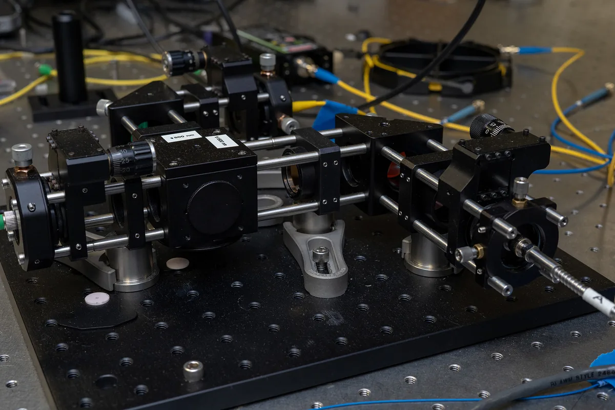
An October 15 preprint reports a two-photon Hong–Ou–Mandel timing experiment that records bunching as well as coincidence outcomes. Its four-detector arrangement reduces dependence on loss calibration in the analyzed estimator and outperforms a two-detector comparison under measured calibration uncertainties. The authors also examine systematic precision floors. Four detectors do not mean four photons, and loss-independent estimation does not mean that photon loss has ceased to reduce the event rate. The result concerns what can be inferred from a richer set of observed outcomes.[1]
Hong–Ou–Mandel interference compares the distinguishability of two photons entering a beam splitter. When their relevant modes match, interference changes the probabilities for finding photons together or in separate outputs. A relative delay alters their overlap, so the outcome distribution can contain timing information. The measurement is not simply a stopwatch attached to each photon. It infers a delay through the statistical pattern generated by interference, which makes source properties, visibility and the detection model part of the inference problem.
Recording only one outcome class can entangle the parameter of interest with a nuisance parameter. A lower coincidence count might reflect a changed delay, fewer generated pairs or greater detection loss. Additional outcomes can help separate those explanations. In particular, observing events in which both photons emerge together provides information that would otherwise be discarded. The appropriate inference uses the joint outcome model. The benefit comes from what those outcomes reveal about the same attempted experiment, not from treating every extra detector as an independent metrological resource.
A deliberately simplified example illustrates cancellation of a common scale factor. Suppose expected counts are N times eta times p for one outcome and N times eta times one minus p for another. Their ratio to the combined count is p, so the common factor eta cancels. This is an invented counting model, not the experiment's complete detector model. If the two outcomes have different unknown efficiencies, the cancellation need not hold. A real estimator must justify the symmetry or calibration relations that make its claimed independence valid.
Even in that simplified model, loss still matters. Reducing eta reduces the total number of detected events. The normalized proportion can remain unbiased while its statistical uncertainty grows because fewer samples survive. Reaching the same precision may then require more source trials or a longer acquisition. This separates two meanings that are easy to confuse: independence from a loss-calibration parameter in the estimator and independence of experimental resource cost from physical loss. The first can be achieved without the second following from it.
Repeated measurements also do not average away every uncertainty. An illustrative error budget can take the form of a statistical variance divided by the number of independent repetitions, plus a fixed systematic variance. Increasing repetitions reduces the first term while leaving the second. Calibration uncertainty shared across a dataset can create such a floor. Correlations between repetitions can further weaken the expected statistical improvement. A precision claim therefore needs to state whether it describes fluctuations within a fixed calibration or uncertainty that includes recalibrating and repeating the complete experiment.
The experiment finds about a twofold precision improvement at the repetitions performed. The authors attribute that gain to the loss-calibration floor: the two schemes have the same statistical dispersion and extract the same information per detected pair. A roughly fourfold separation is a projected comparison as both approach their systematic floors. Changing losses shifts the unrecalibrated two-detector estimate, while the four-detector result remains consistent across the tested conditions.[1]
The study's broader lesson is that useful metrology can come from retaining outcome categories that a simpler setup throws away. The next informative comparison would track precision against total launched pairs, acquisition time and repeated calibration cycles. That would show how the calibration advantage translates into a practical timing measurement. Readers can then distinguish a better inference rule from a brighter source or a less lossy instrument, and understand how all three contribute to the eventual uncertainty in the estimated delay.