
Work through the quantum model.
Follow the amplitudes, operations and resource assumptions. These connected lessons make the calculation visible before a histogram or headline hides its context.
Keep the conventions attached
These are ideal mathematical examples and stated engineering models. Kets use q₀ as the leftmost bit. Angles are in radians unless degrees are named. Read the assumptions before comparing a result with a physical experiment.
Begin with amplitudes and bit order, then follow a worked example. For finite counts, use the 620-in-1,000 shot example. For a representation’s raw storage, use the existing memory calculator.
Complex amplitudes and interference
An amplitude is a complex number. Its squared magnitude gives an outcome probability only in the specified normalized state and measurement basis.
Read the calculation and its limits
Add first, square afterward
Write z = x + iy, where i² = −1. Its squared magnitude is |z|² = x² + y². The polar form r exp(iθ) separates magnitude r from phase θ, the angle from the positive real axis. These are two descriptions of the same number.
For coherent contributions a and b, |a+b|² = |a|² + |b|² + 2 Re(a* b), where the star means complex conjugation. The final term is interference. Adding probabilities alone discards that term and answers a different question.
With a = 1/2 and b = i/2, the combined amplitude is (1+i)/2 and its squared magnitude is 1/2. Replacing b by −1/2 gives zero. Both choices separately have |a|² = |b|² = 1/4. These are contributions to an output amplitude, not necessarily a complete normalized state.
Normalize without changing relative phase
For a nonzero vector (a₀,…,a₍d−1₎), divide every entry by the same factor √(Σⱼ|aⱼ|²). The vector (3,4i) becomes (3/5,4i/5), not an equal superposition. Taking absolute values, discarding imaginary parts or normalizing entries separately changes the intended state.
Multiplying the entire state by exp(iφ) changes only global phase and leaves every measurement probability unchanged. Multiplying one component changes relative phase and can change a later interference measurement even when the current computational-basis histogram stays fixed.
The all-zero vector has no normalized direction. Nonfinite entries are invalid. Large finite entries need a common scaling factor before numerical squaring to avoid overflow; roundoff tolerance is not a license to repair arbitrary invalid inputs.
Read the sources
- IBM Quantum Learning: quantum state vectors and measurements
- John Watrous: states, channels and measurements, Chapter 2
Continue the explanation
Can two states share a computational-basis histogram and still interfere differently?
Yes. That histogram omits relative phase. A later gate can combine amplitudes and reveal the difference.
Vectors, inner products and bit order
Every vector needs basis labels. Here, q₀ is the leftmost bit: |q₀q₁⟩ uses the order |00⟩, |01⟩, |10⟩, |11⟩.
Read the calculation and its limits
Conjugate the first vector
A one-qubit pure state is |ψ⟩ = a|0⟩ + b|1⟩ with |a|² + |b|² = 1. The inner product ⟨φ|ψ⟩ conjugates the entries of φ before multiplying and summing. Without conjugation, imaginary entries can produce an impossible negative self-overlap.
Orthogonal states have zero inner product. Normalized states equal up to global phase have overlap magnitude one. For pure states, |⟨φ|ψ⟩|² is the probability that the projector onto |φ⟩ succeeds on |ψ⟩. It does not measure algorithmic usefulness.
Keep subsystem labels attached
In this ordering, (a,b) ⊗ (c,d) = (ac,ad,bc,bd). Preparing |+⟩ on q₀ and |1⟩ on q₁ gives (0,1/√2,0,1/√2). Reversing the subsystems changes where the nonzero entries appear.
A gate on q₀ is U ⊗ I; a gate on q₁ is I ⊗ U. Applying A first and B second gives BA|ψ⟩. Diagram wire order, amplitude indexing and printed classical strings can follow different conventions even in the same software framework.
Use an asymmetric check: start with |10⟩. CNOT with q₀ controlling q₁ gives |11⟩; CNOT with q₁ controlling q₀ leaves |10⟩ unchanged. A Bell histogram alone can miss reversal because 00 and 11 read the same backward. The three-bit example 110 below provides another check.
An SDK translation requires an explicit permutation from native order to these labeled kets, including the actual classical measurement map. Indiscriminately reversing strings is insufficient when named registers or nontrivial measurement maps are involved. The calculations here do not establish that an SDK adapter was executed.
Read the sources
- IBM Quantum Learning: multiple quantum systems
- John Watrous: states, channels and measurements, Chapter 2
Continue the explanation
Which operation acts on the left qubit in the stated two-qubit ordering?
U ⊗ I acts on q₀. I ⊗ U acts on q₁. The ordering and subsystem labels are part of the calculation.
Observables and finite-shot estimates
A measurement outcome, an expected value and an estimate from finite counts are different quantities.
Read the calculation and its limits
Specify the observable
A Hermitian operator A describes a finite-dimensional projective observable. Its real eigenvalues are possible outcomes, and its orthogonal eigenspaces define the alternatives. An eigenstate makes this observable certain in the ideal model, not every other observable.
For density matrix ρ, the expectation is Tr(ρA). The variance is Tr(ρA²) − [Tr(ρA)]². A pure state can have nonzero measurement variance.
Pauli Z gives +1 on |0⟩ and −1 on |1⟩. For p₀ = 0.36 and p₁ = 0.64, the expectation is −0.28. Because Z² = I, the variance is 1 − (−0.28)² = 0.9216. A single shot returns +1 or −1, never −0.28.
Separate three kinds of uncertainty
With N independent identical shots, the sample mean estimates the expectation and its variance is the single-shot variance divided by N. Its standard deviation therefore scales as 1/√N. More shots do not remove calibration bias or fix an incorrect model.
Outcome randomness describes the specified measurement distribution. Sampling uncertainty describes what finite data establish about it. Model uncertainty asks whether preparation, noise and readout describe the experiment. A narrow statistical interval addresses sampling uncertainty under its assumptions.
Do not multiply estimates of noncommuting observables as though both were jointly measured on each copy. Measuring separate Pauli terms on separate preparations is one way to estimate a Hamiltonian; grouping and covariance can change the sample budget.
Report the observable, eigenvalue convention, counts, estimator and uncertainty procedure. An interval [lo,hi] for p₀ transforms into [2lo−1,2hi−1] for the Z expectation. A probability interval cannot be attached unchanged to a quantity ranging from −1 to +1.
Read the sources
- John Watrous: states, channels and measurements, Chapter 2
- NIST: confidence intervals for a proportion
Continue the explanation
Does a narrower sampling interval certify correct calibration?
No. A biased measurement can yield a precise estimate of the wrong rate. Sampling uncertainty and systematic error require separate evidence.
Pauli operators, rotations and order
The sign, half-angle and units in a rotation formula are part of its meaning.
Read the calculation and its limits
State the matrices and convention
I leaves a qubit unchanged. X exchanges amplitudes. Z changes the sign of the |1⟩ amplitude. Y acts as Y(a,b) = (−ib,ia). X, Y and Z are Hermitian, square to I and have eigenvalues +1 and −1.
For a unit axis vector n and Pauli vector σ = (X,Y,Z), Rₙ(θ) = exp(−iθ n·σ/2) = cos(θ/2)I − i sin(θ/2)n·σ. The angle θ is in radians, with this minus-sign and half-angle convention.
Rz(θ) has diagonal entries exp(−iθ/2), exp(iθ/2). The phase gate P(θ) has entries 1, exp(iθ). They differ by global phase on an isolated target and therefore have the same isolated measurement predictions. Once conditional on another qubit, that phase can become relative between control branches. Controlled-U and controlled-exp(iφ)U need not be equivalent.
Distinguish observable order from global phase
On |0⟩, H then Z produces |−⟩; Z then H produces |+⟩. Their computational-basis histograms match, but an X measurement is deterministically −1 in the first case and +1 in the second.
XZ and ZX differ by a minus sign. On an isolated state, that difference is global and cannot alone be detected by measuring the resulting state. It is not the same demonstration of observable order dependence. A controlled context requires its own phase accounting.
For energy-valued Hamiltonian terms A and B, evolution is exp[−i(A+B)t/ℏ], where ℏ is the reduced Planck constant. Replacing it by exp(−iAt/ℏ) exp(−iBt/ℏ) generally introduces error when A and B do not commute. Shorter repeated steps may reduce approximation error while increasing implementation cost.
A useful circuit explanation names the input, ordered operations, controls, targets and measured observable in text. A diagram must agree with those operations; small gate count and small approximation error are distinct goals.
Read the sources
- IBM Quantum Learning: quantum state vectors and measurements
- John Watrous: states, channels and measurements, Chapter 2
Continue the explanation
Can a phase ignored on an isolated gate matter after adding a control?
Yes. A phase common to an isolated output can become a relative phase between control branches. It must be retained or explicitly compensated.
Measurement, state updates and feedback
A measurement description must distinguish outcome probabilities from what happens to the state afterward.
Read the calculation and its limits
Keep conditional and averaged states separate
For the ideal Lüders projective measurement with projectors Pⱼ, outcome j has probability pⱼ = Tr(Pⱼρ). If pⱼ is nonzero, its conditional state is PⱼρPⱼ/pⱼ. Discarding the outcome record instead gives ΣⱼPⱼρPⱼ.
Measuring |+⟩ in the computational basis and discarding the record yields I/2. Keeping the record identifies |0⟩ or |1⟩ for that run. The average over records is not one definite branch.
A positive-operator-valued measure consists of positive operators Eⱼ that sum to I and specifies probabilities Tr(ρEⱼ). It does not uniquely determine the state update. A measurement instrument is needed; in a simple case, operators Mⱼ satisfy Eⱼ = Mⱼ†Mⱼ and determine the conditional transformation.
Devices can have the same outcome probabilities on selected states but disturb them differently. A classical readout confusion matrix is not a complete physical quantum measurement model.
Feedback follows the measured record
Mid-circuit measurement produces data, classical logic processes the record, and a later operation depends on it. Delay includes acquisition, processing, transport and actuation. A branch after the whole job finishes is not a real-time branch inside the circuit.
In ideal teleportation, the receiver cannot read the unknown input from the local state before receiving the classical result. The correction conditioned on that record recovers the input. Conditional notation does not create faster-than-light communication.
Postselection keeps only runs meeting a condition. Its acceptance fraction and collection cost remain part of the result. Active correction uses information to modify or reinterpret the state. A protocol may use both, but one cannot replace the other in a claim.
Read the sources
- John Watrous: states, channels and measurements, Chapter 2
- IBM Quantum Learning: multiple quantum systems
Continue the explanation
Do outcome probabilities alone specify how a detector changes the state?
No. A POVM specifies those probabilities; a measurement instrument also specifies the state transformation. The projective update above uses the stated ideal Lüders instrument.
From a gate request to physical control
A gate symbol names an intended transformation. The controller must realize it using interactions available on a particular device.
Read the calculation and its limits
Follow the control chain
The path can include compilation, scheduling, calibrated pulse parameters, digital waveform generation, analog conversion and propagation through a physical control chain. Logical intent, scheduled operation, physical control action and measured performance are related descriptions, not interchangeable ones.
For a microwave-driven qubit, in-phase and quadrature envelopes describe components relative to a carrier reference. Their amplitude and phase determine an effective drive in a suitable rotating-frame model. This account is specific to that control model; it is not a universal wiring diagram.
A pulse amplitude or duration needs the device response, frequency, transfer function and calibration procedure. A square waveform at the generator need not remain square at the qubit: filtering, reflections, distortion and unintended coupling can change it.
Calibration connects the request with a response
Rotation-amplitude sweeps, detuning experiments and Ramsey sequences probe particular parameters. A successful isolated-gate calibration does not establish the same error during a simultaneous many-qubit workload.
Some Z rotations use phase-reference updates instead of a separate physical pulse. Within a supported model, this can reduce direct pulse duration. It still requires correct frame tracking, timing and subsequent phases; the compiler and controller must agree on the accumulated frame.
Superconducting, trapped-ion and neutral-atom implementations need separate platform context. An illustrative control chain omits component specifications and cannot establish an achievable error rate. Neither a gate symbol nor a language-supported instruction guarantees backend support or gate fidelity.
Read the sources
- Krantz and colleagues: superconducting-qubit engineering review, version 5 (2021)
- OpenQASM specification: circuit timing
Continue the explanation
Does a calibrated gate duration specify the complete physical operation?
No. Its meaning depends on the device response, waveform, reference frame, calibration and operating context. Performance must be measured in the relevant workload.
Clocks, synchronization and phase
Sample rate, timing jitter, phase noise, latency and fidelity describe different aspects of control.
Read the calculation and its limits
Time is part of the experiment
Operations can overlap, wait for resources or depend on measurement results. Waveform samples, digital logic, acquisition windows and carrier phase may use different clocks whose relationships must be defined.
Sample rate says how often a digital waveform is specified. It is not a measurement of jitter, analog bandwidth, phase noise or gate fidelity. More samples per pulse do not by themselves establish a more accurate physical result.
Make the unit conversion explicit
For carrier frequency f, a time offset Δt gives phase offset Δφ = 2πfΔt. As synthetic arithmetic, 6 GHz × 1 picosecond = 0.006 cycles, or 2.16 degrees. This is a phase offset, not a measured gate error. Infidelity requires the operation, fluctuation statistics and relevant sensitivity model.
A fixed offset may be calibrated. Random fluctuations, drift and correlated offsets have different consequences. A common shift can cancel in one relative measurement but matter elsewhere. A timing result needs its measurement bandwidth and statistical definition.
Respect propagation and decision deadlines
Separate controllers may need shared references, trigger alignment, timestamps and deterministic sequencing. Signals take time to propagate. A measurement-conditioned decision must reach the relevant operation before its deadline; low average network latency does not establish that every decision does.
Optical control raises related synchronization questions but uses different frequencies, components and stabilization methods. The microwave arithmetic above is not an optical phase specification or an invented laboratory tolerance.
A schedule can be syntactically valid without being supported by a real controller. Keep illustrative delays, physical waiting and phase-reference tracking distinct, and distinguish the latency of one result from sustained processing throughput.
Read the sources
- Krantz and colleagues: superconducting-qubit engineering review, version 5 (2021)
- OpenQASM specification: circuit timing
Continue the explanation
Does the 2.16-degree example imply a particular gate infidelity?
No. It converts a stated time offset into carrier phase. A gate-error prediction also needs an operation and a noise-sensitivity model.
Readout and a two-state assignment model
The reported bit is the end of a physical measurement, signal-acquisition and classification chain.
Read the calculation and its limits
Separate the physical signal from its label
A dispersive superconducting-qubit example can include a resonator, amplification, sampling, demodulation and classification. Other platforms can use fluorescence or photon detection. Improving a classifier cannot recover information the physical measurement never distinguished; a strong signal can still be mislabeled through drift or an unsuitable threshold.
Let a be the probability of reporting 1 when 0 was prepared, and b the probability of reporting 0 when 1 was prepared. For true state-1 probability p, the reported rate is y = a + (1−a−b)p. If 1−a−b is nonzero, the unconstrained inverse is p = (y−a)/(1−a−b).
For a = 0.02, b = 0.03 and y = 0.40, p = 0.38/0.95 = 0.40. This coincidence is specific to these inputs and does not make readout errors harmless.
Keep singularity and unphysical estimates visible
If a+b = 1, the reported rate no longer distinguishes p and this inverse is undefined. Near that value, small rate or calibration uncertainties can produce a large change in the inverse. Probabilities must be finite and within their allowed ranges.
Finite data or model mismatch can yield an inverse estimate outside [0,1]. Silent clipping hides this diagnostic. A constrained statistical estimator is a different named procedure, not the same calculation with its result concealed.
Basis-state calibration can include preparation error. The model may miss leakage, simultaneous-readout correlations or drift between calibration and experiment. Multiplying single-qubit assignment matrices assumes a structure that must be tested.
Evaluate on separate data
Training and evaluating a classifier on the same labeled records can overstate performance. Use independent evaluation data, record acquisition conditions and check drift. Retain the confusion matrix when class imbalance matters and carry calibration uncertainty into the corrected estimate.
This arithmetic is a stated classical assignment model, not a full quantum measurement instrument or a hardware calibration. Keep raw rates, assumptions and any correction visible together.
Allow time for the resonator to empty
Correctly assigning a readout label, obtaining the same label again and preserving the intended qubit state answer different questions. A fast classifier does not by itself establish a nondestructive measurement.
In an ideal passive model, photon occupation follows n(t) = n₀ exp(−κt). Here κ is the photon-number decay rate in inverse microseconds, not an amplitude decay rate or κ/2π. The required wait is zero when the target already exceeds the initial occupation; otherwise it is ln(n₀/n_target)/κ.
| Target occupation | Wait (μs) |
|---|---|
| 2 | 0.6770126 |
| 0.2 | 1.252659 |
| 0.02 | 1.828305 |
For a strictly sequential synthetic cycle, a 0.6 μs measurement plus 1.4 μs recovery takes 2.0 μs; a 1.0 μs measurement plus 0.4 μs recovery takes 1.4 μs. The second is faster only for this timing boundary. Readout quality and work that can overlap recovery remain separate.
This model omits active depletion, thermal repopulation and qubit transitions. Nesterov and Pechenezhskiy, version 2, discuss why increased readout power can improve discrimination while also driving unwanted transitions.
A synthetic teaching model. Inputs stay in this page; no device, account or remote computation is used. The worked example remains readable without JavaScript.
Read the sources
- Krantz and colleagues: superconducting-qubit engineering review, version 5 (2021)
- NIST: confidence intervals for a proportion
- John Watrous: states, channels and measurements, Chapter 2
Continue the explanation
Why not silently clip an inverse assignment estimate into [0,1]?
An out-of-range value can reveal finite-data or model problems. Clipping hides that signal; a constrained estimator needs its own definition and uncertainty analysis.
Calibration, drift and T₁/T₂
A lifetime estimate belongs to a sequence, a fitting model, acquisition conditions and a time.
Read the calculation and its limits
Different experiments answer different questions
Relaxation probes how populations approach equilibrium under a stated model. Ramsey probes phase evolution and dephasing. Echo changes sensitivity to some slowly varying disturbances. Gate benchmarking and application tests measure other behavior; one number cannot replace all these experiments.
In a simple zero-temperature relaxation model, excited-state population decays as exp(−t/T₁). A compatible two-level Markovian model can give a coherence envelope exp(−t/T₂) and 1/T₂ = 1/(2T₁) + 1/Tφ. With nonnegative pure-dephasing rate, T₂ ≤ 2T₁.
That relation is not a universal audit rule for every fitted envelope or non-Markovian experiment. Noise can produce non-exponential decay. State the sequence, fit function, uncertainty, operating conditions and measurement time.
Operating context can change
Parameters can drift between calibration and a workload. Recalibration consumes time and resources. Inspect residuals: a poor fit can reflect the wrong model, insufficient data or actual instability, not simply a parameter that needs more digits.
A gate measured alone can behave differently when neighbors are active because of crosstalk, frequency collisions, shared resources or schedule changes. Distinguish isolated and simultaneous tests and state whether the operating point was maintained.
Randomized benchmarking estimates a modeled average under its protocol. It does not certify the worst-case error of every algorithm or reveal every coherent and correlated mechanism. Long coherence does not by itself establish accurate entangling gates, measurement or scalable control.
Read the sources
- Krantz and colleagues: superconducting-qubit engineering review, version 5 (2021)
- Magesan, Gambetta and Emerson: randomized benchmarking methodology
Continue the explanation
Does a long T₁ or T₂ establish the success probability of an application?
No. It diagnoses behavior within its measurement model and operating context. Gates, readout, correlated errors, scheduling and the application need separate evidence.
Decoder latency and throughput budgets
Repeated syndrome records create both sustained processing work and deadlines for particular decisions.
Read the calculation and its limits
Separate rate from delay
A decoder uses syndrome records and a model to infer a correction or update a tracked frame. Throughput is sustained processing rate; latency is the delay before a particular item or decision becomes available. A pipeline can have high throughput and substantial individual latency.
A fast decision on one small case does not show that a decoder sustains a long experiment with many concurrent logical blocks. Some decisions can wait; others must arrive before a dependent operation.
Calculate only the declared fluid model
As synthetic constant-rate arithmetic, suppose an initially empty queue receives 1,000 units per second and processes 900 per second. After five seconds, the backlog is (1,000−900) × 5 = 500 units. With initial backlog Q₀ and constant rates λ and μ, the nonnegative fluid result is max(0,Q₀+(λ−μ)t).
This is a fluid toy model, not a decoder simulation. Real arrivals can burst, syndrome patterns can require different work, and communication, memory movement and dependencies can dominate. Mean service above mean arrivals does not by itself establish acceptable tail latency or remove every risk of growth.
Tie a deadline to a dependency
Tracking a Pauli frame can avoid physically applying every inferred correction immediately. A later operation or interpretation may still depend on that frame. Its deadline comes from the architecture and dependency, not a universal rule that every decode must finish within one syndrome cycle.
A timing benchmark needs the code, distance, concurrent blocks, noise model, syndrome volume, processing hardware and included work. Separate offline replay from live closed-loop operation. Omitting transfer or preprocessing may suit a component benchmark, but those omissions remain relevant to a system claim.
Classical information flow belongs in a logical-computing resource budget alongside qubits and quantum gates. The arithmetic here establishes no operational decoder performance.
Read the sources
- Microsoft Quantum: resource-estimation assumptions
- OpenQASM specification: circuit timing
- Fowler and colleagues: surface-code architecture review (2012)
Continue the explanation
Does high sustained throughput guarantee that a particular correction arrives before its deadline?
No. Throughput and individual or tail latency are different measurements. The relevant decision deadline depends on the operation that consumes the result.
Platform constraints and the whole system
A refrigerator, a vacuum chamber, an optical processor and a semiconductor device are different implementation contexts. No single cutaway represents every quantum computer.
Read the calculation and its limits
Identify the platform
Many superconducting-qubit systems use dilution refrigeration. Trapped-ion and neutral-atom systems use vacuum and optical control, with implementation-dependent details. Photonic systems involve sources, interference, switching and detection. Spin systems can combine semiconductor devices with demanding control and cryogenic requirements.
A system explanation must identify which platform it describes. Illustrative component relationships cannot establish exact vendor dimensions, an engineering bill of materials or attainable error rates.
Trace heat and information separately
In a cryogenic example, cables and components can carry signals and heat. Temperature stages have different purposes and cooling capacities. More channels can create thermal and packaging challenges, while nearby electronics or multiplexing introduce their own tradeoffs. There is no universal cable-per-qubit ratio.
In an optical example, light must be generated, stabilized, delivered, shaped and detected. Loss, mode matching, alignment and detection matter. Encoding information in photons differs from using photons to connect modules of another platform; specify the optical subsystem’s role.
Keep the operational footprint in view
Power supplies, vibration isolation, vacuum equipment, timing distribution, classical processors and calibration can be part of the operating system. A chip photograph is not its complete footprint. A chip metric does not directly establish datacenter energy, cost or performance.
Supporting resources need not all scale linearly with qubit count. Shared equipment, modularity and architectural changes can alter scaling. Identify what is shared, what is per module and what remains unspecified.
Follow storage, control delivery, readout, environmental support and classical feedback. At each step ask what the component does, which limits it introduces and how that behavior is measured. Exact dimensions, component specifications and achieved performance require device-specific evidence.
Read the sources
- Krantz and colleagues: superconducting-qubit engineering review, version 5 (2021)
- Bruzewicz and colleagues: trapped-ion engineering review (2019)
- Saffman, Walker and Mølmer: Rydberg-atom review (2010)
- Knill, Laflamme and Milburn: linear-optical computation (2000)
Continue the explanation
Can a chip-level metric be used directly as a whole-system energy or cost comparison?
No. The operational system includes control, readout, environmental support and classical work, with architecture-specific sharing and scaling assumptions.
Logical runtime and resource assumptions
A logical-qubit count alone determines neither runtime nor the full physical machine.
Read the calculation and its limits
Begin with a task and an error budget
A resource estimate needs a target result, precision, acceptable failure probability, circuit construction, error-correction approach and scheduling model. Data storage is only part of the resources: ancillas, routing, resource-state factories, buffers and spare capacity can matter.
T count is the number of T operations. T depth is the number of sequential layers under a stated scheduling and ancilla model. A resource-state factory has an output rate, footprint, error characteristics and startup behavior. Enough data qubits do not guarantee that states arrive when needed.
Keep separate lower bounds separate
As synthetic planning arithmetic, one million required resource states and a combined supply of 1,000 acceptable states per second imply at least 1,000 seconds for supply alone, ignoring startup and buffering. If dependency-constrained execution requires 2,000 seconds, that is a separate lower bound.
The larger bound is 2,000 seconds, but taking the maximum is not a complete schedule. Overlap, contention, interruptions and state availability still need modeling. This example is not a device runtime prediction.
Carry the assumptions through the conclusion
Allocate failure probability among memory, gates, preparation, measurement, approximation and other mechanisms. The union bound gives P(any failure) ≤ Σⱼpⱼ without requiring independence. Multiplying survival probabilities requires additional assumptions and is not automatic.
Code distance depends on the workload and error model. A phenomenological scaling formula teaches conditional trends, not decoder- and circuit-specific performance. Correlated faults and architecture constraints can invalidate extrapolation from one physical-error rate.
Vary dominant assumptions such as operation time, logical failure model, factory rate, routing overhead, precision and algorithm construction. Preserve the baseline and distinguish a lower bound, a modeled schedule and measured execution. Historical resource estimates retain their dates and assumptions; they are not automatically the current best estimate.
Average output can hide a shortage
Both supply and demand total 18 accepted states over these six synthetic slots. Start empty; receive supply, discard any overflow, serve that slot’s demand, then record the remaining stock. Unserved demand is counted as a shortage and is not carried forward.
| Slot | Supply | Demand | Discard | Short | Stock |
|---|---|---|---|---|---|
| 1 | 3 | 0 | 0 | 0 | 3 |
| 2 | 3 | 1 | 0 | 0 | 5 |
| 3 | 3 | 8 | 1 | 1 | 0 |
| 4 | 3 | 0 | 0 | 0 | 3 |
| 5 | 3 | 0 | 0 | 0 | 6 |
| 6 | 3 | 9 | 2 | 2 | 0 |
At capacity 7, three states are discarded and three are missing when needed. Capacity 10 removes both losses for this exact sequence. The same average production rate therefore supports different schedules depending on storage.
This inventory model omits state fidelity, aging, routing and factory failures. A code rate k/n converts logical demand to physical data qubits by division by k/n; checks, factories, buffers and interfaces are additional resources. The dynamic-pipeline study’s buffer analysis illustrates why storage and stalls belong in a full resource estimate.
A synthetic teaching model. Inputs stay in this page; no device, account or remote computation is used. The worked example remains readable without JavaScript.
Read the sources
- Microsoft Quantum: resource-estimation assumptions
- Gottesman: stabilizer codes and fault-tolerant operations (1997)
- Fowler and colleagues: surface-code architecture review (2012)
Continue the explanation
Does taking the maximum of supply and dependency lower bounds produce a complete runtime schedule?
No. It gives a necessary lower bound under the stated assumptions. A schedule must also model state availability, overlap, contention, startup and interruptions.
Worked example: normalize (3,4i)
Use the basis |0⟩, |1⟩. This is an exact mathematical example, not a reconstructed physical state.
Read the calculation and its limits
Normalize and read the probabilities
The conjugate of 4i is −4i, so |4i|² = 16. The squared norm is 9 + 16 = 25, and the norm is 5. Dividing both entries by 5 gives |ψ⟩ = (3/5)|0⟩ + (4i/5)|1⟩.
The amplitudes are (0.6,0.8i); computational-basis probabilities are (0.36,0.64). Their magnitude ratio is 3:4, and the second amplitude has relative phase π/2. Replacing 0.8i with 0.8 keeps these probabilities but changes the state.
Multiplying the whole vector by i gives (0.6i,−0.8), an equivalent pure state. Imaginary amplitudes still matter: a common phase is unobservable, while a phase difference can alter later interference.
Construct the density matrix
The outer product |ψ⟩⟨ψ| is [[0.36,−0.48i],[0.48i,0.64]]. Its trace is one and determinant zero. In ρ = (I+xX+yY+zZ)/2, the upper off-diagonal entry is (x−iy)/2. Thus (x,y,z) = (0,0.96,−0.28). Its squared length is 0.9216 + 0.0784 = 1.
The sign matters: y = −2 Im(ρ₀₁), not +2 Im(ρ₀₁). A computational-basis histogram cannot reveal the wrong sign.
Apply H before squaring
H(a,b) = ((a+b)/√2,(a−b)/√2). Here the output is ((3+4i)/(5√2),(3−4i)/(5√2)); both squared magnitudes are 25/50 = 1/2. Balanced probabilities do not imply equal or real amplitudes.
Normalizing (3,4) instead gives the same initial 0.36:0.64 histogram. After H, its probabilities are 49/50 and 1/50. The difference comes from relative phase.
Normalization and applying the Born rule to an already normalized state are separate operations. An all-zero vector cannot be normalized, and nonfinite inputs are invalid. An ideal arithmetic result is not evidence of a physical gate or a tested SDK implementation.
Read the sources
- IBM Quantum Learning: quantum state vectors and measurements
- John Watrous: states, channels and measurements, Chapter 2
Continue the explanation
Why does replacing 4i by 4 change the Hadamard result but not the initial histogram?
The initial computational-basis measurement loses relative-phase information. H combines amplitudes before their magnitudes are squared, so it reveals that phase difference.
Worked example: a density matrix and Bloch vector
Compare a pure state, an incoherent mixture and I/2 without inferring the full state from one histogram.
Read the calculation and its limits
Form the projector with a conjugated row
Let |ψ⟩ = (√3/2)|0⟩ + (i/2)|1⟩. Its probabilities are 3/4 and 1/4. The outer product gives ρ = [[3/4,−i√3/4],[i√3/4,1/4]]. Use the conjugate transpose, not an ordinary transpose.
For ρ = (I+xX+yY+zZ)/2, x = 2 Re(ρ₀₁), y = −2 Im(ρ₀₁), and z = ρ₀₀−ρ₁₁. The Bloch vector is (0,√3/2,1/2). Its length is one, and the Y expectation is positive √3/2.
For a valid one-qubit state with Bloch length r, eigenvalues are (1+r)/2 and (1−r)/2. Here they are 1 and 0. Purity is Tr(ρ²) = (1+r²)/2 = 1. Base-two von Neumann entropy is −Σⱼλⱼ log₂λⱼ = 0 bits, using the continuous convention 0 log₂0 = 0.
Remove coherence without changing the histogram
Setting the off-diagonal entries to zero gives diag(3/4,1/4). Its Bloch vector is (0,0,1/2), purity 5/8 and entropy approximately 0.811278 bits. The computational-basis probabilities are unchanged, but the ideal Y expectation is now zero.
For I/2, the Bloch vector is zero, eigenvalues are 1/2 and 1/2, purity is 1/2 and entropy is one bit. Many pure-state ensembles give this same density matrix; it does not carry a uniquely determined hidden surface point.
A globally pure Bell state has local density matrix I/2 on either subsystem. Local entropy does not mean that the global state was a classical mixture.
Require positivity
The matrix [[1/2,0.6],[0.6,1/2]] is Hermitian with trace one, yet its eigenvalues are 1.1 and −0.1. It is not a physical density matrix. Plausible diagonal probabilities are insufficient: the matrix must also be positive semidefinite.
Small numerical excesses within a stated tolerance can be roundoff. Substantial violations cannot be silently repaired as though the input were unchanged. Any projection or state-reconstruction procedure is a separate estimator.
Read the sources
- John Watrous: states, channels and measurements, Chapter 2
- IBM Quantum Learning: multiple quantum systems
- John Watrous: quantum entropy, Chapter 5
Continue the explanation
Can the pure state and diag(3/4,1/4) be distinguished by a single 75:25 computational-basis histogram?
No. They share that histogram. A Y-basis measurement distinguishes their ideal predictions: √3/2 versus zero. Trace one and Hermiticity alone also do not certify a physical density matrix.
Worked example: multiply X, Y, Z and H
Start with |ψ⟩ = (3/5,4i/5). Its complex entries expose sign and phase errors that a real-only example may hide.
Read the calculation and its limits
Multiply rows by the state vector
In the basis |0⟩, |1⟩: X = [[0,1],[1,0]], Y = [[0,−i],[i,0]], Z = [[1,0],[0,−1]], and H = [[1,1],[1,−1]]/√2. Multiply the matrix by the amplitudes before taking squared magnitudes.
X|ψ⟩ = (4i/5,3/5), exchanging the computational-basis probabilities. Y|ψ⟩ = (4/5,3i/5); the first entry is positive because (−i)(4i/5) = 4/5. Z|ψ⟩ = (3/5,−4i/5), changing relative phase while preserving the current histogram.
H|ψ⟩ = ((3+4i)/(5√2),(3−4i)/(5√2)), with outcome probabilities 1/2 and 1/2. Comparing only those probabilities can miss a wrong phase.
Check invariants and order
X² = Y² = Z² = H² = I. Applying any one twice recovers the state. Unitaries preserve normalization and inner products; numerical checks require a stated tolerance.
On |0⟩, H then Z gives |−⟩, while Z then H gives |+⟩. Both have 50:50 computational-basis probabilities. An X measurement gives −1 for the first and +1 for the second.
XZ versus ZX alone gives only a global minus sign on an isolated target. The operator algebra is noncommuting, but that particular output difference alone is not observable. Adding control changes the phase accounting.
Separate arithmetic from SDK or hardware evidence
An SDK comparison must map its basis ordering explicitly and compare states up to global phase where appropriate. Component-by-component comparison can reject equivalent vectors; probability-only comparison can accept inequivalent vectors.
These hand calculations and reference arithmetic describe ideal mathematical gates. They do not certify device noise, compilation or an arbitrary backend. No physical-device execution or executed SDK adapter is demonstrated in this lesson.
Read the sources
- IBM Quantum Learning: quantum state vectors and measurements
- John Watrous: states, channels and measurements, Chapter 2
Continue the explanation
Why check complex amplitudes before checking a histogram?
A histogram omits relative phase. Distinct states can give identical probabilities in one basis while behaving differently after another gate or in another measurement basis.
Worked example: bounded CHSH correlations
This is an ideal state-and-measurement calculation. It is not a physical loophole-free Bell test or an apparatus certificate.
Read the calculation and its limits
Define the expression before evaluating it
Use |Φ+⟩ = (|00⟩+|11⟩)/√2. Restrict local observables to the X–Z plane: A(a) = cos(a)Z + sin(a)X and B(b) = cos(b)Z + sin(b)X, with outcomes +1 or −1. In this model E(a,b) = cos(a−b), with angles in radians.
Choose S = E(a₀,b₀) + E(a₀,b₁) + E(a₁,b₀) − E(a₁,b₁). Local hidden-variable models under the relevant locality and setting-independence assumptions obey |S| ≤ 2.
Set a₀ = 0, a₁ = π/2, b₀ = π/4 and b₁ = −π/4. The correlations are, respectively, 1/√2, 1/√2, 1/√2 and −1/√2. Therefore S = 2√2 ≈ 2.828427. Each correlation is within [−1,1]; this is below the algebraic maximum 4 and reaches the quantum bound.
Add one named noise assumption
Let ρ(v) = v|Φ+⟩⟨Φ+| + (1−v)I₄/4, where 0 ≤ v ≤ 1. The maximally mixed term has zero correlation for these traceless observables, so E is multiplied by v. At the chosen settings S = 2√2v.
For v = 0.8, S ≈ 2.262742. The chosen expression exceeds 2 when v > 1/√2. This statement is confined to this state family and these measurements. No violation here does not prove separability or certify a device as classical.
Nonfinite angles and visibility outside [0,1] are invalid. The stated model cannot exceed |S| = 2√2. At v = 0 all four correlations vanish. The sign convention for S must remain explicit.
Identify the missing experimental evidence
A physical estimate needs counts for all setting pairs, a setting-selection protocol and a statistical analysis. Detection, timing, independence and data selection affect the interpretation. Favorable postselection without accounting for its procedure can alter the claim.
Matching 00 and 11 in one basis can also arise from a classical mixture. Choosing a visibility value sets a model assumption; it does not measure entanglement. Exact or synthetic model output does not establish loophole closure, device independence or communication security.
Read the sources
Continue the explanation
Does setting v = 0.8 verify entanglement in a real device?
No. It assumes a particular mixed-state model and computes its correlations. An experimental claim needs measured data, a protocol and analysis of the relevant loopholes and assumptions.
Worked example: why CNOT does not clone |+⟩
One fixed linear operation cannot make perfect independent copies of every arbitrary unknown quantum state.
Read the calculation and its limits
Apply the proposed copier to a superposition
Suppose U copies computational-basis inputs into a blank target: |0⟩|0⟩ becomes |00⟩ and |1⟩|0⟩ becomes |11⟩. CNOT with q₀ controlling q₁ does this for that orthogonal set.
For |+⟩|0⟩ = (|00⟩+|10⟩)/√2, linearity gives (|00⟩+|11⟩)/√2. Two independent copies would be |+⟩|+⟩ = (|00⟩+|01⟩+|10⟩+|11⟩)/2. The actual output lacks the |01⟩ and |10⟩ terms.
Their overlap is 1/√2 and squared pure-state fidelity is 1/2. They are not related by global phase. For general a|0⟩+b|1⟩, encoding gives a|00⟩+b|11⟩; two copies would require coefficients a², ab, ab and b². A fixed linear map cannot produce that nonlinear dependence for every unknown input.
State the boundaries of the theorem
Known states can be prepared repeatedly from a classical description. A specified orthogonal set can be distinguished and copied. Approximate cloners can optimize a stated approximation. None is a universal perfect copier of an arbitrary unknown state.
Classical bits encoded in orthogonal states can be copied within that basis. The obstruction is maintaining every coherent relationship for unrestricted unknown quantum states; it is not a temporary hardware imperfection.
Encoding and transfer are different operations
Repetition encoding maps a|0⟩+b|1⟩ to a|000⟩+b|111⟩, not three independent copies. Suitable parity measurements can diagnose a restricted class of errors without learning the logical amplitudes. Measuring each physical qubit to recover a and b would destroy the protected coherent state.
Teleportation consumes the original input in its measurement protocol and uses shared entanglement plus classical communication. It does not leave a second intact copy at the sender. Copying, encoding, preparation and transfer must remain distinct.
Read the sources
- Wootters and Zurek: A single quantum cannot be cloned
- John Watrous: states, channels and measurements, Chapter 2
Continue the explanation
Does CNOT clone |+⟩ because it copies |0⟩ and |1⟩ into a blank target?
No. On |+⟩ it creates a Bell state. Copying a specified orthogonal set does not make an unrestricted unknown-state copier.
Worked example: superdense coding with its resource costs
Alice holds q₀ and Bob holds q₁ of a previously shared |Φ+⟩ pair. The two-bit message m₀m₁ and decoded ket both use q₀ as the leftmost bit.
Read the calculation and its limits
Encode all four messages
Start with |Φ+⟩ = (|00⟩+|11⟩)/√2. Alice applies X on q₀ when m₁ = 1, then Z on q₀ when m₀ = 1. Thus messages 00, 01, 10 and 11 use I, X, Z and ZX, respectively.
The resulting states are: 00 → (|00⟩+|11⟩)/√2; 01 → (|01⟩+|10⟩)/√2; 10 → (|00⟩−|11⟩)/√2; 11 → (|01⟩−|10⟩)/√2. These are mutually orthogonal Bell states. Reversing X and Z in the last isolated encoding changes only global phase.
Bob’s local reduced state is I/2 for every message. He cannot read Alice’s choice from q₁ alone. Alice must transmit q₀ before he can make the joint decoding measurement.
Decode after transmission
Once Bob holds both qubits, he applies CNOT from q₀ to q₁, then H to q₀. The four encoded states become |00⟩, |01⟩, |10⟩ and |11⟩, respectively. Computational-basis measurement returns m₀m₁ in this ideal model.
Checking only 00 and 11 can hide reversed labels. The asymmetric messages 01 and 10 distinguish the encoding rules and output ordering.
Count the full communication resources
The protocol uses one previously distributed entangled pair, one transmitted qubit after the message is chosen, local operations and a joint measurement. “Two classical bits with one qubit” requires the entanglement assistance to be stated. Creating and distributing the shared pair was not free.
If establishing that pair is part of the same physical-channel workflow, include its cost together with storage, loss, synchronization and error handling. The elementary result does not give two classical bits per unassisted one-qubit channel.
The distant marginal before transmission does not reveal a readable message, so the protocol does not signal faster than light. A noisy implementation induces a four-message classical channel; retain per-message errors and preparation costs alongside an average success rate. Ideal arithmetic does not measure that channel.
Read the sources
- Bennett and Wiesner: original entanglement-assisted communication paper
- IBM Quantum Learning: superdense coding protocol
Continue the explanation
Which resource makes the two-bit message possible with one transmitted qubit?
A previously shared entangled pair, followed by the transmission of Alice’s qubit and a joint measurement. The prior pair and its distribution costs are part of the resource ledger.
Worked example: recover the secret 110
Bernstein–Vazirani concerns a precisely specified oracle problem. Its n-versus-one exact deterministic query comparison is not an end-to-end practical speedup claim.
Read the calculation and its limits
Define the oracle and ordering
A hidden n-bit string s defines fₛ(x) = s·x modulo two. A standard bit oracle maps |x⟩|b⟩ to |x⟩|b xor fₛ(x)⟩. Preparing the target in |−⟩ gives phase kickback: |x⟩ receives (−1) raised to fₛ(x), while the target factor remains unchanged.
In the exact deterministic classical query model, n independent queries are sufficient and necessary to identify an arbitrary n-bit secret: query strings with a single 1 to reveal its bits. The ideal quantum construction uses one oracle query under the corresponding quantum-access assumptions.
An explicit known-secret teaching circuit has gates determined by s. Giving that secret to the compiler is not discovering it. Oracle construction, target preparation, other gates and physical execution are distinct from query count.
Follow an asymmetric three-bit example
Set n = 3 and s = 110, with the leftmost bit labeled q₀. Start in |000⟩ and apply H to each qubit. All eight basis amplitudes become 1/√8.
In basis order 000, 001, 010, 011, 100, 101, 110, 111, the phase oracle gives signs +, +, −, −, −, −, +, +. Reversing the secret would change this pattern and the final state.
After the final Hadamards, the amplitude of |y⟩ is 2⁻ⁿ times the sum over all x of (−1) raised to [(s xor y)·x]. For y = s, all terms are +1 and the amplitude is 1. If y differs in any bit, the terms pair with opposite signs and cancel.
The output is |110⟩, with probability one in the ideal model. Predict the string before revealing it, and inspect the phase signs before the last Hadamards: the cancellation in amplitudes explains the result.
Bound the conclusion
The query comparison must use the same problem and compatible oracle access, rather than charging unlike implementation work to only one side. The explicit known-secret oracle has O(n) gate structure; one query is not one operation for the whole workflow.
The n-versus-one comparison here is not exponential and does not solve arbitrary hidden-data problems. It uses the special linear form of fₛ. A tiny ideal example or locally checked reference calculation does not demonstrate practical advantage over a classical computer.
No physical-device execution or executed SDK adapter is demonstrated here. A software translation must retain the named bit ordering and test asymmetric strings such as 110, not rely only on symmetric examples.
Read the sources
- Bernstein and Vazirani: Quantum Complexity Theory
- IBM Quantum Learning: Bernstein–Vazirani problem and query analysis
Continue the explanation
Does one oracle query mean the complete application costs one gate?
No. The query model counts access to a defined oracle. Constructing it, preparing states, applying the other gates, compiling and running a physical circuit have their own costs.
For the next reading route, return to the execution glossary and QubitWire’s short reading routes. Source passages and local reference arithmetic checked 1 October 2026. This guide does not claim an executed SDK adapter, physical-device validation or independent scientific replication.
Read the deeper explanation · about 6 min
This estimate covers the explanation below, separate from the overview. Optional depth was added in this reading edition. The article keeps one canonical address and its original chronology. Source review: . The relevant source dates and limitations are recorded below.
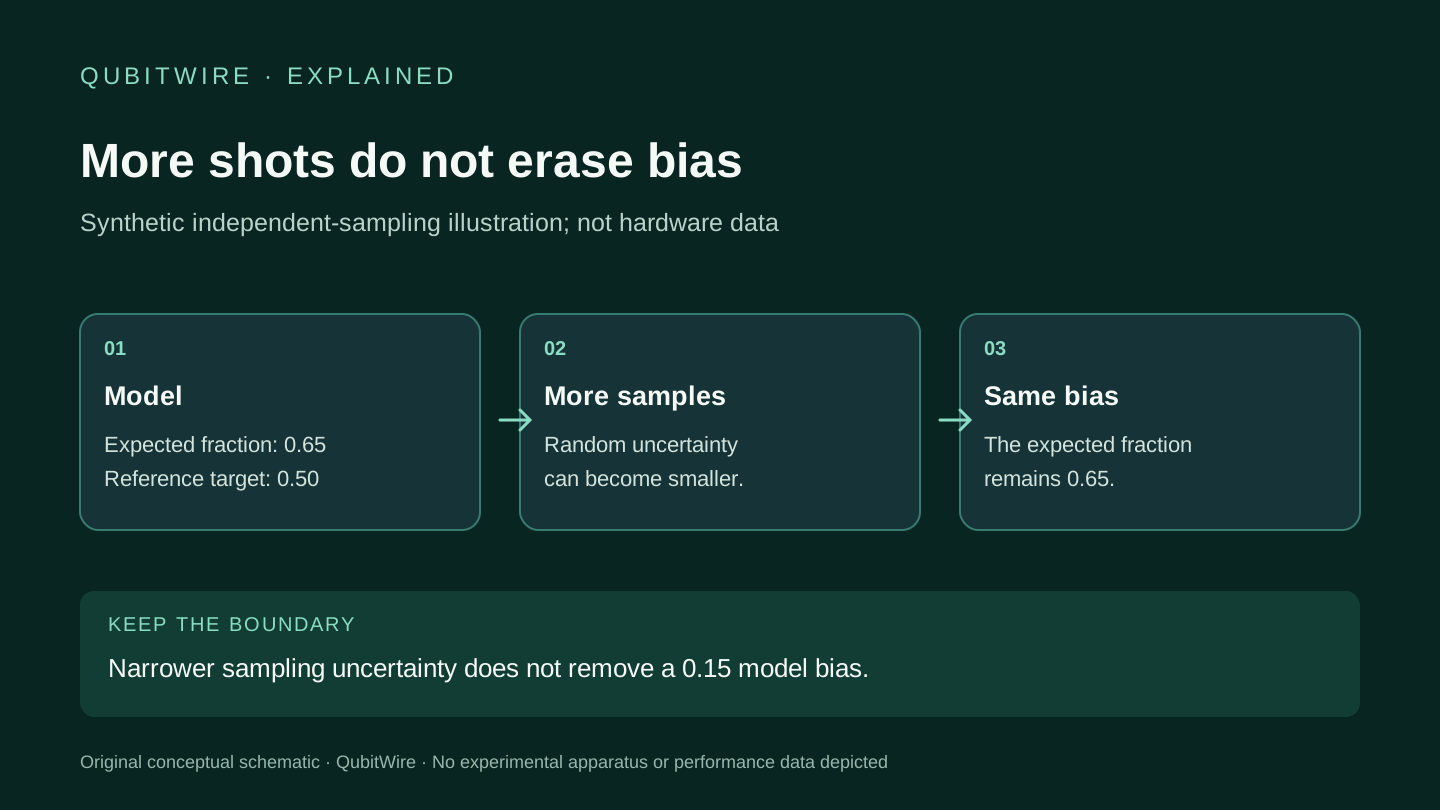
A result can become more precise without becoming more accurate. That distinction is familiar in measurement science, but it is easy to lose when a quantum-computing story emphasizes how many times an experiment was repeated. A large number of shots can be useful evidence. It is not a universal cure for error.
The key is to ask what the repetitions are estimating and which assumptions connect that estimate to the conclusion. Random sampling uncertainty, systematic effects, correlated errors and changes over time are not the same problem. Collecting more data can help with some of them while leaving others largely intact.
What a shot actually gives you
In a simple quantum-circuit experiment, a shot is one execution and measurement under the specified procedure. Repeating the procedure produces a collection of outcomes. The distribution of those outcomes can be used to estimate a probability or another quantity of interest.[1]
That description does not mean every shot is an identical, independent draw from a perfectly stable process. Whether those assumptions are appropriate is part of the experimental question. The hardware, preparation, measurement or environment may change. Data processing can also introduce dependencies that deserve attention.[1][2]
For a beginner, the most useful mental model is not a machine revealing a hidden answer one digit at a time. It is an experiment whose observations support a statistical estimate. The estimate has a meaning only in relation to the procedure used to obtain it.
The biased coin that explains the trap
Imagine a hypothetical instrument intended to report whether a fair coin landed heads or tails. Suppose the instrument sometimes mislabels tails as heads. Running the experiment many times can give a very precise estimate of what the instrument reports. It does not automatically give an accurate estimate of what the coin did.
The analogy is not a model of all quantum noise. It separates two ideas. Sampling uncertainty concerns variation in an estimate because only a finite number of observations was collected. A systematic effect concerns a persistent difference between the thing being measured and the thing being reported or inferred. More observations can make the persistent difference look more convincing if the model ignores it.
Quantum experiments have their own preparation, operation and measurement effects. A report that treats every uncertainty as though it shrinks simply by adding shots risks overstating what the data establish.[1][2]
Correlation can change how much information a dataset contains
A million observations are not necessarily equivalent to a million independent pieces of information. If observations share a source of variation, their dependence can affect the uncertainty of the estimate. The relevant issue is the structure of the dependence, not merely the size of the file.
For example, an experiment that drifts between operating regimes can produce a large pooled dataset that hides the variation across time. Looking only at the pooled average may conceal a behavior that matters for a real application. An analysis that assumes stability should explain why that assumption is reasonable or investigate the consequences when it is not.
A reader does not need to calculate an effective sample size to recognize the question. Ask whether the source examined performance across the run, across relevant settings and across repeated experimental sessions. A single aggregate number can be informative, but it cannot display every form of instability.
A narrow error bar is not a complete uncertainty budget
An uncertainty statement should identify what it includes. Does the interval describe sampling variation under a particular model? Does it incorporate calibration uncertainty? Does it reflect variation between repeated runs? Does it account for the transformation used in error mitigation? These choices affect interpretation.[2]
Two papers can report different-looking intervals because they are summarizing different sources of uncertainty. That is not automatically evidence that one is more careful or more successful. The comparison becomes meaningful after the quantities and methods are aligned.[2]
The clearest wording is specific. Say what was estimated and how the uncertainty was characterized. Avoid translating an interval into a broader probability claim that the source did not establish. Precision in language is particularly valuable when the visual presentation makes an estimate look definitive.[2]
Mitigation is an analysis choice, not an eraser
Error mitigation can use additional measurements, modeling or extrapolation to estimate a quantity less affected by certain errors. Its usefulness depends on the method and the conditions. It can introduce additional sampling cost or rely on assumptions that should be examined. It should not be described as if all physical errors were simply removed from the device.[3]
A well-explained result distinguishes the raw measurement record from the mitigated estimate. It also states the resource cost and uncertainty of the procedure. An attractive final number is only part of the evidence. Readers should be able to see the relationship between the experiment performed and the quantity inferred.[2][3]
This is not an argument against sophisticated analysis. It is an argument for making the analysis visible. Scientific instruments routinely require calibration and inference. Confidence is strengthened when those steps are documented and tested, not when they are hidden behind a 'noise-free' label.
How to make the next chart more informative
A quantum-computing chart can communicate much more than a single mean. Depending on the experiment, useful views might include variation over time, the distribution across instances, comparison of raw and processed estimates, or sensitivity to an important analysis choice. The right chart is the one that helps answer the stated question.[1][2]
The display should identify the number of trials or instances where relevant, the meaning of error bars, any excluded data and the source of the comparison. Axes and baselines should not be chosen to imply a larger practical difference than the underlying task supports. These are design decisions with scientific consequences.
For an educational site, a simple interactive example can make the central point. Let a reader increase the number of simulated shots while separately controlling a small measurement bias. The sampling cloud tightens as observations accumulate, but the biased center remains displaced. Label the simulation as illustrative and keep its assumptions visible. Do not make the toy model look like a live hardware benchmark. This is a proposed teaching design. The existing Noise Lab changes a phase-flip probability and sample count; the bias example in this reading edition is a fixed table.
What would actually strengthen the evidence?
The answer depends on the concern. More independent observations can improve a sampling estimate. A calibration experiment can help characterize a measurement effect. A changed experimental design can test a suspected confounder. Independent implementation can probe whether a conclusion depends on one particular setup.[1][2]
The useful next step is therefore targeted, not simply larger. A bigger dataset is valuable when it addresses the uncertainty that limits the claim. It is less informative when it repeats the same blind spot with greater numerical precision.
A responsible article can say this without implying that the researchers have made a mistake. Every experiment has a scope. The job is to explain which questions the design answers and which questions remain open.
The number to remember is not a number
There is no universal shot count at which a quantum result becomes trustworthy. The relevant standard depends on the quantity, the procedure, the uncertainty model and the claim being made. A small carefully designed experiment can answer one question well. A very large dataset can answer a different question poorly.
When the next headline celebrates millions of measurements, ask what those measurements made more certain. Did they narrow random sampling uncertainty? Did they characterize the system's behavior across changing conditions? Did they test the assumptions behind the estimate?
More data can be powerful. The most useful confidence comes from knowing what the data actually say.
Evidence for this explanation
- A Quantum Engineer’s Guide to Superconducting Qubits — version 5
Review first submitted April 13, 2019; this version revised July 7, 2021. Complete primary HTML checked October 11, 2026. Historical preparation, control, readout and calibration context; no current device result is claimed.
- NIST statistical handbook: confidence intervals for proportions
Primary handbook text and Wilson formula checked October 11, 2026; no page publication date inferred. Sampling intervals require their statistical assumptions and do not silently include unknown readout bias, drift or arbitrary correlation.
- IBM Quantum documentation: error mitigation and suppression techniques
Complete primary documentation checked October 11, 2026. Additional calibration circuits, repeated noisy runs, model-based extrapolation and sampling overhead; mitigation is not guaranteed to produce an unbiased result. No implementation or hardware job was run.