 Context photo · Holger Muench / IBM · CC BY 2.0Open video to choose privacy settingsFundamentals7:17
Kurzgesagt – In a Nutshell001
Context photo source & license
Expert explainers, lab tours, interviews, and technical deep dives—curated for clarity and substance.
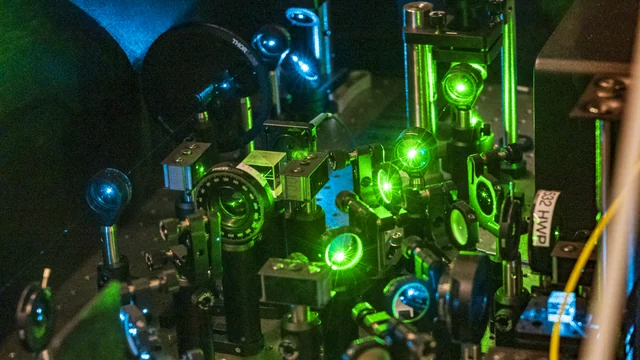
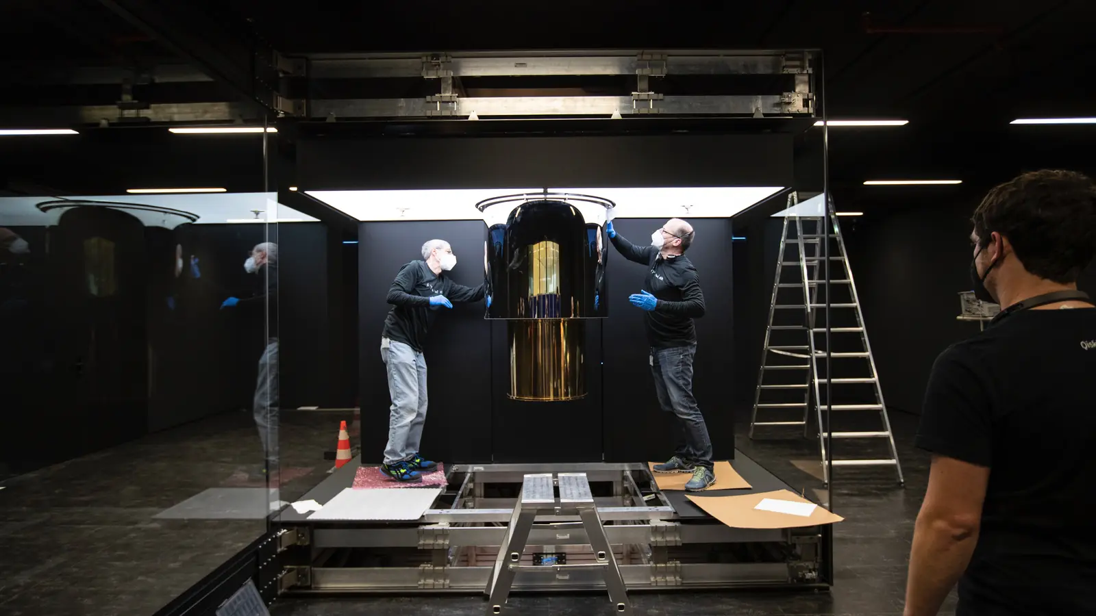
Context photographs illustrate each subject; they are not video frames. Photo sources & licenses.
Local photos are shown until you allow YouTube previews.
Clear titles, trusted channels, and every subject in one compact index.
Ordered by recorded YouTube views; counts may change.
Context photo · Holger Muench / IBM · CC BY 2.0Open video to choose privacy settingsFundamentals7:17 Context photo · ORNL · CC BY 2.0Open video to choose privacy settingsFundamentals24:28
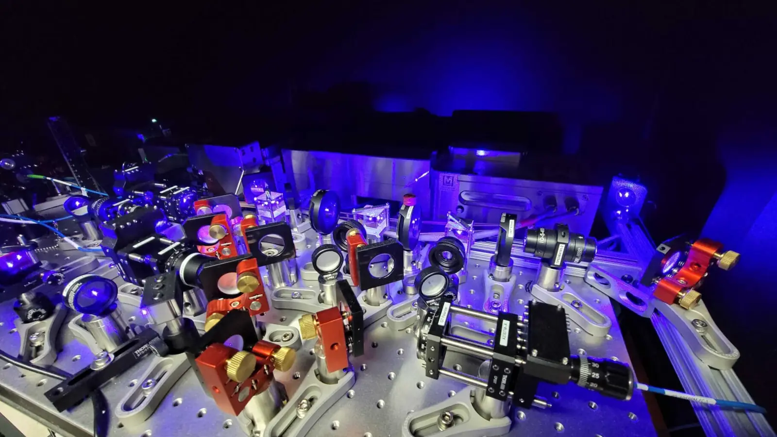 Context photo · QuEra · CC BY 4.0Open video to choose privacy settingsExplainers17:00
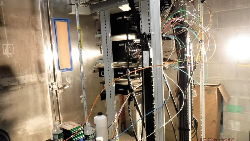 Context photo · MTA Capital Construction Mega Projects · CC BY 2.0Open video to choose privacy settingsIndustry24:01Context photo · ORNL · CC BY 2.0Open video to choose privacy settingsQuantum Culture11:51Context photo · ORNL · CC BY 2.0Open video to choose privacy settingsExplainers53:57Context photo · Holger Muench / IBM · CC BY 2.0Open video to choose privacy settingsHardware11:58Context photo · Holger Muench / IBM · CC BY 2.0Open video to choose privacy settingsFoundations17:34Context photo · ORNL · CC BY 2.0Open video to choose privacy settingsExplainers19:27Context photo · Holger Muench / IBM · CC BY 2.0Open video to choose privacy settingsResearch4:42Context photo · Holger Muench / IBM · CC BY 2.0Open video to choose privacy settingsFundamentals6:47
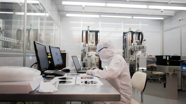 Context photo · Lucy Knowles / UC Davis College of Engineering · CC BY 2.0Open video to choose privacy settingsHardware12:23
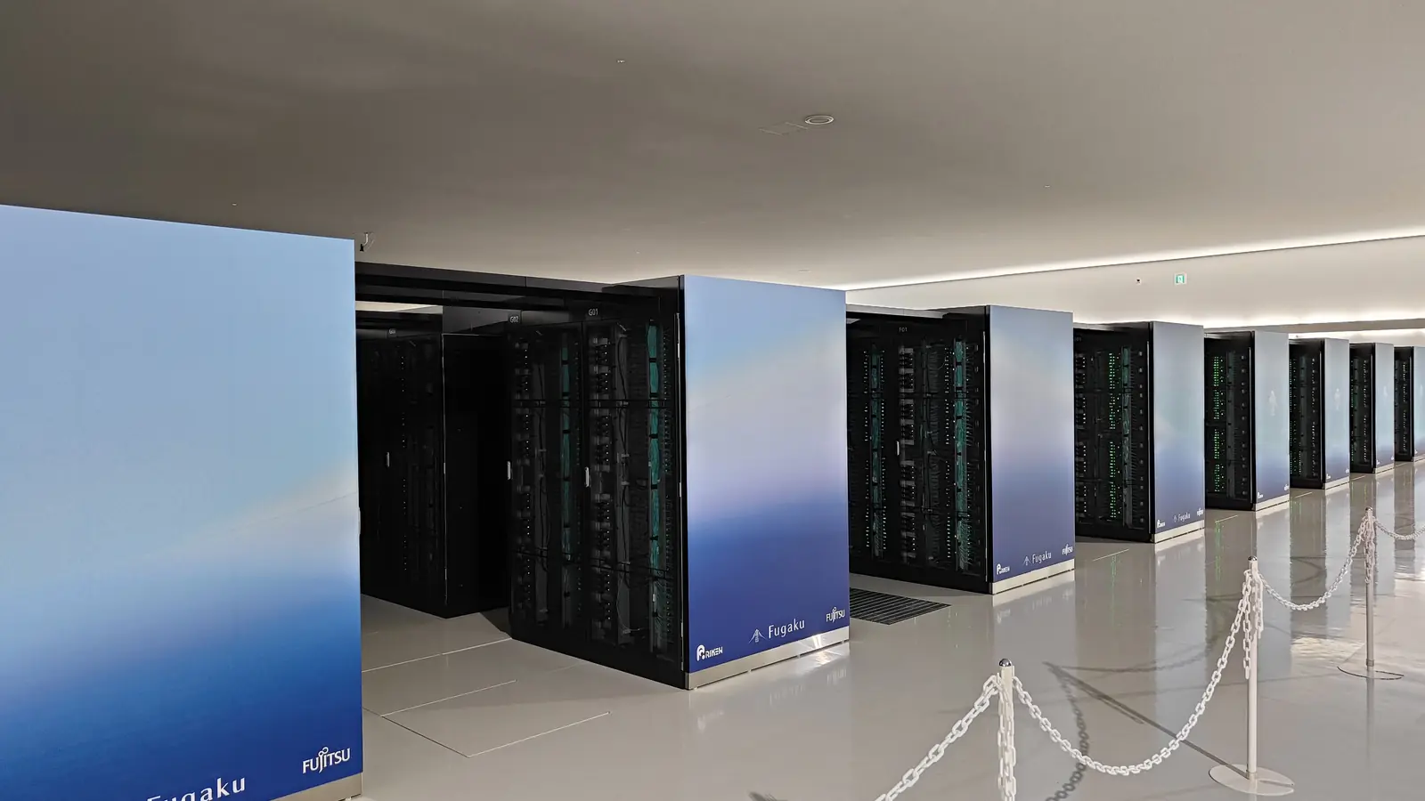 Context photo · Barsaka2 · CC0 · CC0 1.0Open video to choose privacy settingsAlgorithms36:54Context photo · Holger Muench / IBM · CC BY 2.0Open video to choose privacy settingsIndustry8:35Context photo · Holger Muench / IBM · CC BY 2.0Open video to choose privacy settingsCourses1:56:28Context photo · Holger Muench / IBM · CC BY 2.0Open video to choose privacy settingsTantalum-on-silicon superconducting qubits2:20
16 of 262 videos
Choose a question, use it alongside a video already in the library, then follow the source reading. These learning notes offer a way to inspect an explanation; they do not certify every claim made in a recording.
What apparatus or procedure is actually shown? What result is measured? Keep those two questions separate when a laboratory tour moves between real equipment and a simplified picture.
An animation can explain an idea without establishing that a device exists. A tour can show hardware without demonstrating every claim made about it. Compare what you see with the original source’s description of the setup and its measured result.
Original QubitWire viewing questions. Source reading:
Laboratory, fabrication and systems-engineering context. This page does not certify every assertion in the recording.
Institutional page; checked 11 October 2026.Open existing library video: Step inside the Google Quantum AI lab — Google Quantum AI.
Follow one instruction through the system: a description of an operation reaches control hardware, acts on the quantum device and eventually contributes to a measurement or later decision. Ask what each step does, rather than treating every cable and electronic box as interchangeable.
This background route concerns superconducting circuits. Other architectures use different controls. The accompanying review introduces superconducting-qubit design, control, noise and readout; it helps identify the jobs around the chip without claiming that the tour demonstrates a complete fault-tolerant computation.
Original QubitWire viewing questions. Source reading:
Official article links this exact IBM laboratory recording and describes processor-characterisation context.
Article published 18 December 2024.Background on superconducting-qubit design, noise, control and readout; specific architecture, not a universal equipment description.
Review published 2019; arXiv v5 revised 7 July 2021.Open existing library video: Lab Tour: How IBM tests quantum processors — IBM Research.
When an algorithm is called faster, ask which task it performs and what it receives as input. Preparing data, accessing it, choosing an accuracy and extracting the answer can all change the useful comparison.
Scott Aaronson’s 2015 commentary uses quantum linear-system algorithms to make those conditions concrete. Treat it as a historical reading companion, then compare any current advantage claim with a classical method doing the same task under comparable assumptions.
Original QubitWire viewing questions. Source reading:
Input preparation, access assumptions, conditioning, output extraction and fair classical comparisons in quantum linear-system algorithms.
Commentary published in Nature Physics on 2 April 2015.Publication identity and date. The linked author-hosted manuscript provides an accessible reading copy.
Commentary published 2 April 2015.Open existing library video: Quantum Algorithms Pt.3 Tracking Advantage | Minh Tran | QGSS26 — Qiskit.
Use these statistical questions alongside a discussion of quantum noise. If a result has error bars, first find their definition: do they describe sampling, variation between runs or another uncertainty model?
A narrow interval can still miss a persistent measurement bias. More independent observations can reduce sampling uncertainty without repairing that bias. Ask which effects the uncertainty calculation includes. These questions do not assume that this recording contains a particular chart.
Original QubitWire viewing questions. Source reading:
Binomial-proportion intervals and the role of sample size; relevant to appropriately modelled counts.
Handbook reference; publication date not stated.Distinguishes measurement uncertainty, precision and bias, and accounts for random and systematic contributions.
Handbook reference; publication date not stated.Open existing library video: Explaining quantum noise | Tools for Quantum Advantage | Ep2 — Qiskit.
Open the source behind the central claim. IBM’s official episode page supplies the superconducting and cryogenic context for this conversation. It describes systems engineering needed to house, cool and operate processors, alongside future plans.
Check the date and type of evidence behind each statement. A cooling-system milestone, a measured processor result and a forecast for an interconnected machine answer different questions. Follow the linked announcement before treating a programme’s intended destination as something already demonstrated.
Original QubitWire viewing questions. Source reading:
Exact episode title, superconducting context, cryogenic engineering and linked announcements; company context remains attributed.
Episode information; publication date not stated.Open existing library video: Why IBM quantum computers are colder than space — IBM Research.
Build your understanding
Four pathways through six video referrals and eight course collections. Open the provider page for current access and playback. These resources are separate from the video library above.
Start with conversations about what quantum computing can do and the questions still open.
John Preskill and Brian Greene discuss quantum mechanics and the direction of quantum computing.
Caltech points readers to a conversation about Preskill’s path into quantum information and the field’s evolving direction.
A historical lecture that explains the promise and limits of noisy intermediate-scale machines.
Move from explanations and provider demonstrations to a structured technical course.
An architecture-specific explanation of error correction from the company developing the parity approach.
A demonstration linked from Riverlane’s APS recap showing an end-to-end error-correction workflow.
A provider-led discussion of the engineering milestones behind quantum error correction, with a presentation and industry panels.
A structured course on protecting quantum computations from noise through error-correcting codes and fault tolerance.
Explore practical access and the relationship between quantum and high-performance computing.
A practical starting point for learning the basics and beginning to use quantum-computing resources.
Learning material on combining quantum and high-performance computing within one workflow.
Compare algorithmic ideas with the work of planning and evaluating a quantum project.
A course exploring quantum approaches to matrix diagonalization and related algorithm families.
A structured introduction to using quantum-computing methods within machine learning.
A course on the variational quantum eigensolver and chemistry-oriented examples.
Business-oriented learning material introducing quantum technology and potential applications.
A course for teams planning and managing early quantum initiatives.
Provider pages checked 24 September 2026. Referral dates are not new upload dates.
From recent events
These links lead to the organizers’ own pages. Check availability and playback there.
Sessions held October 10–18 cover quantum programming, research and applications. The organizer lists seven recordings.
GESDA’s October 27 report page includes a video of workshop participants discussing access to quantum computing and its potential public benefits. Read the report alongside the discussion to distinguish proposals from delivered outcomes.
Open the GESDA report and video →Organizer pages checked October 27, 2026. Session and report dates are not video upload dates.
Source reading
44 independent lessons unpack the ideas behind official quantum recordings, with questions, exercises and primary reading.
Learning routes include official lessons, seminars and archives. Each guide has a preparation step and a concrete follow-up exercise; a gateway is distinct from a single recording.
PennyLane’s official tutorial material links to a Variational Quantum Eigensolver video and provides a current written route into related methods. This learning plan uses that official connection to study a precise question: how does the chosen family of trial states shape the answer an optimiser can find? The video is an existing educational resource, with an accompanying preparation and review exercise. Its official source route was verified; playback, captions and duration were not independently checked.
Before opening the recording, write down the three components of a small variational problem: the operator whose expectation value is measured, the parameterised state preparation and the classical rule that updates parameters. Keep these components separate on the page. A low reported energy could result from an expressive trial family, a fortunate initial point or a carefully chosen tiny problem. It should not be treated as evidence that every stage will behave similarly for a larger scientific task.
During the viewing session, use a two-column notebook. In one column, record what the ansatz preserves or restricts, such as an explicitly stated symmetry or a fixed circuit pattern. In the other, record what freedom remains for the optimiser. Pause when a parameter changes and explain which physical or mathematical state change it permits. The purpose is to turn a sequence of code cells into a model of the search space. If the recording uses an older interface, follow its mathematical argument and consult current documentation before adapting its syntax.
For the follow-up, choose a small Hamiltonian whose exact spectrum can be computed classically. Compare two justified trial families under an equally documented optimisation budget. Record initial conditions, evaluations and stopping rules. A family that cannot represent the desired state can fail even when the optimiser is working correctly. Conversely, a sufficiently expressive family does not guarantee that a particular optimisation run will find the best point. Keep representational limits and search failures visible as separate explanations for the observed result.
Identify the measured operator, the trial-state family and the classical update rule. Each can limit the result for a different reason.
No. It is one outcome under a particular search budget. Compare against a small exact reference and examine both representational restrictions and optimisation history.
Source identity and written learning context reviewed. No independent playback, caption assessment or completed exercise is claimed.
Official VQE video identity
Playback, captions and runtime not tested.
Official referring page links the VQE video and related written material
Written tutorial updates may use APIs different from the recording.
Quantum Machines’ official video page describes a Qolab demonstration of automated superconducting-qubit calibration performed remotely on a device in Madison. The source presents it as a live conference demonstration and names a sequence of calibration activities. This learning route treats that account as a vendor-hosted description and asks the reader to inspect the workflow’s decisions. The demonstration is vendor-hosted. Playback was not independently assessed.
Prepare by drawing four boxes: acquire data, estimate a parameter, decide whether to accept it and validate the resulting setting. Then leave room for an unsuccessful branch after each box. Automation becomes easier to understand when these decision points are visible. A script that moves smoothly from one experiment to the next may still need rules for incomplete data, a poor fit, an unexpected parameter or a failed validation. The useful viewing question is which of those rules is actually shown and which remains outside the presentation.
When the recording is accessible, take notes on one calibration stage rather than attempting to document every screen. Identify the raw observable, the analysis method and the setting changed as a consequence. Record any stated acceptance threshold exactly with its context. If the video does not disclose a threshold, mark it unspecified. Avoid inferring it from a green indicator or a successful-looking curve. The difference matters because a viewer may later want to reproduce the decision, not merely produce a similar plot.
For a follow-up exercise, create a synthetic example in which the fitted parameter moves but the validation result worsens. Explain what an automated workflow should do under an explicitly chosen policy. Retain the previous accepted setting, the candidate setting and the reason for the decision. This is a proposed learning case rather than a claim about Qolab’s actual implementation. It helps distinguish estimating a parameter accurately from improving the operation that the calibration is meant to support.
The data used, estimate, acceptance rule, candidate value and validation result. The setting alone does not preserve the reasoning that made it acceptable.
Record that boundary. Do not assume the system lacks it, but do not invent a policy that the source has not documented.
Source identity and written learning context reviewed. No independent playback, caption assessment or completed exercise is claimed.
Vendor-hosted video description of remote Qolab calibration demonstration
Demonstration account is attributed; no independent playback or reliability assessment.
Quantum Machines’ on-demand seminar page describes adaptive estimation of superconducting-qubit frequency and relaxation behaviour, followed by feedback or feed-forward intended to improve operation. The official abstract provides the topic and research context; playback and the numerical performance statements were not independently assessed. The learning route focuses on the relationship between a changing physical parameter, the evidence used to estimate it and the action taken afterwards.
Begin with an ordinary estimation problem: a quantity changes over time, while each measurement is noisy and costs something to obtain. Write down how an old estimate can become less useful even if it was precise when measured. Then distinguish the timescale of the underlying change from the time needed to acquire data and compute an update. These relationships are more informative than the word real-time on its own. A fast computation can still arrive too late if the measurement or communication stage dominates the complete loop.
When the seminar is available, use a timeline to organize the explanation. Mark preparation, interrogation, readout, inference and application of the new setting. For each claimed improvement, identify which part of that timeline was measured and which comparison was used. Keep the estimator’s uncertainty separate from the uncertainty of a downstream gate or coherence measurement. A method can track a parameter more efficiently without automatically improving every operation that depends on it. The source’s own validation evidence should determine the scope of the conclusion.
For a follow-up exercise, simulate a small drifting scalar parameter with occasional jumps. Compare a fixed measurement schedule with an explicitly defined adaptive schedule under the same observation budget. Report tracking error, delay after a jump and the cost of the chosen updates. Do not present the synthetic signal as a realistic transmon model unless that additional assumption is supported. The exercise is intended to make the tradeoff visible, including situations where adaptation responds too slowly or overreacts to noise.
Its age must be considered relative to how quickly the relevant quantity changes and how long the complete update loop takes. Precision at measurement time is only part of that assessment.
No. The downstream operation needs its own validation under the updated setting. The learning note should preserve that separate evidence.
Source identity and written learning context reviewed. No independent playback, caption assessment or completed exercise is claimed.
Official on-demand seminar gateway; adaptive estimation and feedback subject
Abstract performance claims attributed; no independent validation, playback or access-form test.
Qblox’s Quantum Builders page provides an official webinar route on building silicon-spin quantum processors. Its accompanying discussion addresses fabrication, wiring, individual device variation and moving electrons between locations. This is a source-hosted technical conversation, not a neutral certification of a hardware roadmap. The new learning route asks readers to connect those topics through the interfaces that a complete processor requires. The recording is existing material; playback and captions were not independently checked for this volume.
Before viewing, make a simple map with four layers: fabricated device, electrical access, calibrated operation and application-level task. Place each statement from the conversation at the layer it actually concerns. A lithographic pattern belongs to a different evidence category from a measured operation, and an operation on a small selected device is different from a manufacturing yield distribution. This map helps a newcomer understand why progress in one layer can be substantial without resolving every challenge in the layers above it.
Pay particular attention to connections. When the discussion mentions a wire, gate electrode, control channel or movement between sites, ask what information or physical action crosses that boundary. Then ask how the boundary is characterized. A geometric drawing may show that a route fits, while electrical measurements establish whether the signal arrives with acceptable distortion and noise. A shuttling demonstration can establish a specific transport operation without proving that an entire future architecture has been integrated. Keep the scale and conditions attached to each example.
The follow-up exercise is an interface ledger for a hypothetical small spin-qubit experiment. List the input supplied to each layer, the output expected and the test that would detect a failure. Use illustrative values only when labelled as such; there is no need to invent device specifications. One useful row might connect a software voltage request to the actual calibrated device setting. Another might connect a physical operation to the measurement used to judge it. The ledger should reveal where a claim depends on evidence not present in the source.
A fabricated structure and a measured qubit operation establish different things. The connection between them requires tuning, readout and a defined test, with yield assessed over an appropriate population.
Use it to understand the questions and interfaces. A cross-platform ranking would require matched tasks and comparable evidence beyond one sponsor-hosted discussion.
Source identity and written learning context reviewed. No independent playback, caption assessment or completed exercise is claimed.
Official webinar gateway and discussion of wiring, fabrication, variation and shuttling
Sponsor-hosted conversation; projections are not integrated-system achievements.
Zurich Instruments hosts a webinar page on tune-up workflows with the LabOne Q applications library, supported by an official tutorial collection. This route is designed for readers who see automated experiment software and want to understand what each stage actually establishes. The source pages confirm the educational route and software context. They do not establish that the replay plays in every browser, that every example matches the current release or that a tune-up was independently executed on a device.
Prepare a worksheet with one row for each kind of experiment encountered: the physical question, the varied control, the measured output and the inferred parameter. Keep the worksheet focused on one small chain of dependencies. An automated workflow may make several experiments look like a single button, but the scientific meaning still resides in the individual measurements and assumptions. The reader should be able to explain what would happen if one stage produced ambiguous or inconsistent data.
During the viewing session, look for the boundary between a reusable workflow and a device-specific calibration. A library can provide a structure for acquisition and analysis, while the actual configuration, parameter ranges and acceptance decisions still depend on the setup. Record where the presentation supplies those details and where it leaves them to the operator. Do not treat a default value in a demonstration as a universal recommendation. A useful note identifies the reason a parameter is chosen and the evidence that would justify changing it.
For the follow-up, take one tutorial workflow and describe its inputs and outputs without copying its entire implementation. Then add a hypothetical failed fit or inconsistent validation. Explain which later steps depend on the missing or rejected result. This exercise should remain a written design review unless the reader has a suitable, authorised environment for execution. A successful software import is not a successful calibration, and a plotted curve should not be labelled as measured hardware data when it was generated synthetically for the exercise.
Only after checking why it was chosen and whether it fits the intended device and experiment. A tutorial default is part of an example, not a universal operating specification.
The workflow needs an explicit decision tied to its purpose. The learning exercise should show which downstream steps depend on that result and preserve the failure rather than silently continuing.
Source identity and written learning context reviewed. No independent playback, caption assessment or completed exercise is claimed.
Official webinar route for LabOne Q tune-up workflows
Replay, registration conditions and captions not tested.
Companion workflow tutorials
Pin the software release before adapting examples.
MIT OpenCourseWare’s archived 8.05 Quantum Physics II course includes a video lecture continuing its treatment of two-state systems and an official gallery of lecture recordings. This route uses the archive to strengthen a foundational skill: keeping track of the basis when separate quantum systems are described together. The course is identified as Fall 2013 material. The new contribution is this guided exercise, not a claim that the lecture is recent or that its playback and captions were independently tested.
Before opening the lecture, write a normalized state for one two-state system and another for a second system. Expand their product in an explicitly ordered basis. Choose an order and keep it visible beside every vector or matrix. Much confusion in introductory quantum software comes from switching conventions without noticing. A component’s position in a printed vector does not identify a physical outcome until the basis order is known. This is a small calculation worth doing by hand before relying on a library.
Use the viewing session to connect notation with questions that can be answered operationally. Which probabilities would be obtained by measuring one subsystem? Which quantities require a joint description? When an operator acts on only one part, identify the identity operator that accompanies it on the other part. The learning goal is not to memorize a larger matrix. It is to understand why the larger representation has the structure it does and how the chosen ordering affects the way that structure is written.
For the follow-up, compare one product state with a clearly defined correlated state. Compute a small set of measurement probabilities and explain which similarities do not establish that the states are the same. Then change the basis order and show that the physical predictions remain unchanged when the transformation is handled consistently. This proposed exercise can be completed with pencil and paper or a small matrix calculation. It should not be presented as an entanglement experiment on a physical device or as a test of a commercial quantum processor.
The entries acquire physical meaning through that order. A silent change in ordering can make a correct calculation look wrong or a wrong interpretation look plausible.
Generally not. The exercise should distinguish the information supplied by a chosen measurement from a complete state description.
Source identity and written learning context reviewed. No independent playback, caption assessment or completed exercise is claimed.
Official lecture-video resource
Archive educational source; playback and captions not tested.
Official course lecture gallery
No claim that all recordings have equivalent accessibility or current player support.
IBM Quantum Learning’s stabilizer-formalism lesson provides an official video, companion slides and written material on Pauli operators and stabilizer codes. This route uses that lesson to answer a foundational question: how can an error-correction procedure learn about an error without simply reading out the logical information it is meant to protect? The official lesson and its YouTube destination were verified. Playback, captions and the accuracy of any automatically generated transcript were not independently assessed.
Prepare by writing two small Pauli products and checking whether they commute. Explain the result in words before expanding it into matrices. Then distinguish an operator used to define a code space from an operator that acts on the encoded information. The notation can look similar while the role is different. A clear learning note should state what is being measured, what its possible outcomes mean and which degrees of freedom remain available to carry the protected state.
When watching the lesson, follow one small code example all the way through. Record its stabilizer generators, the allowed code space and a few possible errors. For each error, determine the changed measurement signs. Avoid treating the syndrome as a complete description of everything that happened. Different errors can lead to the same syndrome, and the decoding decision requires the code structure and an error model. The lesson is a route to understanding that reasoning, not evidence that a particular commercial processor has achieved fault tolerance.
The follow-up exercise is a hand-checkable syndrome table. Include at least one pair of errors that illustrates an ambiguity or equivalence relevant to the chosen code. Explain the distinction between detecting that something is inconsistent with the code space and deciding what recovery to apply. A small table is sufficient if the reasoning is transparent. Do not add a fabricated hardware error rate to make the exercise appear experimental. If a simulator is used, retain its assumptions and state that the data is synthetic.
Not generally. Multiple errors can have the same syndrome. A recovery decision depends on the code and assumptions about likely errors.
It keeps the protected information visible in the reasoning and helps distinguish a check outcome from an operation on the encoded state.
Source identity and written learning context reviewed. No independent playback, caption assessment or completed exercise is claimed.
Companion to the existing recording; its original upload date is unchanged.
Official lesson, Pauli observables, stabilizer-code scope and video link
Educational content; not a hardware performance claim.
Exact official-linked video identity
Playback and captions not independently tested.
IBM Quantum Learning’s quantum-algorithmic-foundations lesson explicitly contrasts query-model reasoning with computation on inputs supplied in an ordinary explicit form. Its official page links a lesson video and written material on computational cost. This route asks the reader to preserve the input model whenever an algorithmic advantage is discussed. The source and official-linked video identity were checked; playback, captions and the current player’s accessibility were not independently tested during this source review.
Begin with a simple task and write down how the algorithm receives its input. Is the data already stored in a structure the algorithm can query, produced by a physical system or supplied as an ordinary list of numbers? Then state which operations the cost model counts. These choices are part of the problem definition. A result that reduces the number of calls to a black box can be mathematically strong while leaving the cost of building or implementing that black box unresolved for a particular application.
During the lesson, keep separate columns for input length, number of counted operations and the cost of an individual operation. A number’s value and the number of bits needed to represent it are different quantities. That distinction matters when interpreting whether a cost grows polynomially or exponentially. Use a tiny arithmetic example to make the convention concrete. The goal is to connect asymptotic language to an explicit representation rather than translating every complexity statement into a predicted number of seconds on current hardware.
For the follow-up, choose a short algorithm description and rewrite its resource claim under two clearly stated access models. Identify which work moves outside the counted boundary and which remains inside. Do not invent a speedup ratio or assume that state preparation is free. If the complete implementation cost is unknown, name the missing evidence. A well-formed question about the input interface can be more valuable than a numerical estimate assembled from unrelated gate times, memory assumptions and idealized oracle calls.
No. It answers a precise mathematical question about access and counted resources. Applying it to a concrete workflow requires checking whether that access model can be supplied at the assumed cost.
Algorithms operate on representations. Complexity is often expressed in the length of that representation, which can grow much more slowly than the numerical value.
Source identity and written learning context reviewed. No independent playback, caption assessment or completed exercise is claimed.
Companion to the existing recording; its original upload date is unchanged.
Query versus explicit-input models and computational-cost framing
Asymptotic costs are not wall-clock predictions.
Exact official-linked video identity
Playback and captions not independently tested.
CERN openlab’s account of the first Quantum Technologies for High-Energy Physics conference directs readers to official recordings on the conference website. The event took place on November 1–4, 2022. This is therefore an archive-learning route, not an upcoming event listing or a report of newly released results. The official recording gateway was verified, while individual replay availability, captions and durations remain untested. The new contribution is a structured way to compare what different quantum methods are being asked to do.
Start by choosing one task category rather than treating quantum technology as a single application. A sensing proposal, a simulation method, an algorithm and a communication system solve different kinds of problems. Write the desired output in ordinary language. It might be an estimated physical quantity, a distribution, a reconstructed event or a secure transfer primitive. Then identify the existing method used to obtain that output and the limitation that motivates the proposed quantum approach. This prevents a broad institutional programme from being mistaken for one integrated machine.
When exploring the archive, select one talk whose title and abstract match the chosen task. Keep the date attached to every claim. Record whether the presentation describes a theoretical proposal, a numerical study, a laboratory result or a deployment plan. Follow any paper link for the details required to assess the result. A conference recording can explain motivation and context especially well, but a spoken overview may omit assumptions, unsuccessful cases or the exact comparison protocol needed for a technical conclusion.
The follow-up exercise is a task-to-evidence sheet. State the input, required output, accuracy target, classical reference and physical or computational resources. Identify one bottleneck that the quantum component addresses and one that it leaves unchanged. For a sensing example, this might mean distinguishing the sensor response from the complete inference pipeline. For a computing example, it might mean separating a kernel operation from data preparation and validation. These are proposed analytical categories, not a summary of a particular unreviewed talk.
The required output and current bottleneck determine what improvement would matter. Different quantum methods can be relevant for entirely different reasons.
No. Its date and evidence class must remain visible. Current software, access or deployment claims need a fresh source beyond the historical presentation.
Source identity and written learning context reviewed. No independent playback, caption assessment or completed exercise is claimed.
CERN confirms the archive route. Direct retrieval of the Indico destination failed, so individual recordings and playback availability remain unverified.
Four research areas and official direction to conference recordings
Historical programme account; individual talks not independently watched.
Official conference identity and archive gateway
Individual recording access, captions and duration require checking.
NIST’s official video page hosts an animation explaining the NIST-F4 atomic fountain clock and its role in calibrating timekeeping references. The page records an upload date of September 23, 2024. This learning route retains that historical date and the source’s identification of the animation. It does not treat the word newest in the original title as a continuously verified ranking, and it does not claim that playback or captions were tested during preparation of this volume.
Begin with two separate questions: how long is a second, and what time does a clock display? A frequency reference addresses the rate at which cycles are counted; a timekeeping system must also maintain continuity and relate readings to a chosen timescale. Write those roles on a simple chain before watching. This makes it easier to understand why a sophisticated atomic experiment can be essential even when it is not the device directly displaying the time on a wall or a phone.
When the animation is accessible, follow the interaction between atoms, an applied signal and the measured response. Identify which part supplies a physical reference and which part is adjusted to agree with it. The visible animation is an explanatory representation, not documentary footage of every process at its actual scale. Keep that distinction in any caption or classroom reuse. A moving dot or enlarged apparatus component can clarify an idea while still requiring a separate source for the instrument’s measured uncertainty and operating conditions.
For the follow-up, draw a conceptual calibration chain with an independent oscillator, a reference measurement and a correction to the oscillator’s estimated rate. Explain how uncertainty enters the comparison and how an interruption differs from a systematic rate offset. Avoid making up a numerical uncertainty for NIST-F4. A small illustrative example can use clearly hypothetical values to show why repeated measurements reduce some uncertainties while leaving other effects to be modelled or bounded. The exercise concerns interpretation, not a new clock-performance calculation.
The reference helps establish or calibrate a rate. Maintaining and distributing a time reading also requires continuous counting and a timescale relationship.
It should retain its animation label. Explanatory scale, motion and simplification are different from a photograph or a measured data record.
Source identity and written learning context reviewed. No independent playback, caption assessment or completed exercise is claimed.
Official explanatory animation and time-reference context
Original title uses newest; no current ranking inferred. No playback or uncertainty-value verification.
Quandela’s official documentation page lists Perceval and Cloud webinar material, and the company’s learning hub provides a current route into photonic computing and Perceval. The retrieved documentation page repeats several catalogue entries and does not expose a confirmed direct replay link for the named webinar. This record therefore remains a curated research route with an explicit replay hold. It is not a verified playable-video listing. The original learning worksheet below remains useful alongside the official written material.
Start by describing a photonic computation through input, optical transformation and detection. Record whether the input is a photon occupation pattern, a qubit encoding or another explicitly defined state representation. Then write what an output sample means under the chosen detector model. These decisions determine how a circuit’s visual layout connects to the probabilities returned by a simulator or experiment. A reader should not assume that every optical mode corresponds to one qubit or that every detected event is an accepted computational result.
If the official replay is later located and checked, use the worksheet to follow one small example. Record the software version, circuit definition, execution environment and output interpretation. Separate simulator results from remote hardware results, and keep the service’s access conditions dated. A historical webinar can teach a durable concept while using interfaces or cloud offers that have changed. Do not reproduce old access claims as current availability, and do not infer a complete hardware run merely from a demonstration of submission code.
The follow-up exercise is to reconstruct the small example in a documented simulation environment and audit its denominators. State which outcomes are retained, how many attempts are represented and what is lost through selection or an explicitly modelled loss process. This links the viewing plan to the Perceval career pathway without repeating that pathway’s full project. The worksheet’s role is to help a learner recognize the relevant decisions in a presentation and connect them to a reproducible written example. No simulation or hardware experiment was executed for this record.
The official learning gateway and original worksheet are useful, but they must be labelled as a resource brief. A video card should wait until the exact recording and access conditions are checked.
No such conclusion is supported. This packet treats them as repeated source-page content and does not count or promote them as separate recordings.
Source identity and written learning context reviewed. No independent playback, caption assessment or completed exercise is claimed.
The official hub does not establish distinct playable recordings. This is a written learning brief with a source link.
Official catalogue lists Perceval and Cloud webinar material
Repeated entries and no confirmed direct replay; do not infer catalogue count or playable status.
Current official photonic and Perceval learning gateway
Individual course access and hardware availability not verified.
The QuTiP project describes its Virtual Lab as a browser-based graphical environment for exploring simple quantum systems, with tutorial videos and prebuilt examples included in the application. The official introduction and launch destination were verified. The application’s individual videos, playback, captions and runtime behaviour were not independently tested during this source review. This learning route therefore points to an official tutorial-supported environment while keeping its untested interaction details explicit. It is new guidance around an existing project resource.
Begin with a prediction before changing a control. Choose one simple system and write what you expect a selected observable to do when one parameter changes. Name the initial state, the parameter and the observable in the same sentence. This prevents an attractive animation from becoming a substitute for understanding the model. A prediction can be qualitative: faster oscillation, a shifted equilibrium or a change in a decay envelope. Its value lies in being specific enough that the displayed result could disagree with it.
When the tutorial videos are accessible, use them to identify the model behind the interface. Ask which equation or rule governs the evolution, which units the controls use and which environmental effects are included. A graphical control can conceal a modelling assumption as effectively as a line of code. Record the assumption rather than treating the interface as a direct representation of any real laboratory device. If the application does not expose a needed numerical setting, note that limit before drawing conclusions about convergence or physical accuracy.
For the follow-up, vary one parameter while preserving the rest of the configuration. Compare the result with the original prediction and explain any discrepancy. Then choose a limiting case that can be checked independently, such as a vanishing interaction or an explicitly simplified initial condition. The exercise is a proposed learning sequence; no particular configuration is claimed to have been run. A screenshot alone would not preserve the full model, so the reader should also record the configuration and the meaning of the plotted axes.
The initial state, parameters, units, observable and relevant model assumptions. Those details explain what produced the display and what it means.
No. It illustrates the model’s output. Independent limiting cases and numerical checks help assess the computation; physical applicability requires evidence about the intended system.
Source identity and written learning context reviewed. No independent playback, caption assessment or completed exercise is claimed.
This is a virtual-lab gateway with included tutorials, not one recording. Individual playback, captions and runtime were not assessed.
Official description of graphical lab and included tutorial videos
Application interactions and individual tutorial playback not independently tested.
Official launch destination linked by project introduction
Dynamic application content not established by text retrieval; no specific video title or duration claimed.