A benchmark is a measurement or estimate under specified conditions. Its value depends on the task, the definition of success and the resources included. A score may describe an important capability without establishing an advantage for another task.
Keep the denominator in view: circuit size, repetitions, accepted outputs, elapsed time and classical processing can change what the headline number means. Identify whether the result came from hardware, simulation or a projection before comparing it with another result.
A fair application comparison uses an appropriate classical baseline and accounts for the full workflow. That includes work outside the quantum circuit when it matters to the conclusion. A selected demonstration, a theoretical complexity result and a practical operational benefit answer different questions.
Use the QUOPS analysis below as a current case study, then follow the evidence record and fair-comparison guide. The goal is to understand the claim precisely enough to say what additional evidence would support a broader conclusion.
One concept. Choose your depth.
The one-minute explanation
A quantum benchmark measures a particular capability under stated conditions. Read the task, the success rule and the resources counted before interpreting its score.
A larger circuit, a faster run and a useful application are different conclusions. The same number cannot answer every question.
Keep this limit in view: A benchmark alone does not establish an advantage on a different task. A company assessment and a stock return measure different things.
IBM’s QOBLIB update describes a shared library of ten optimization problem classes for comparing quantum and classical methods.
A benchmark library is not evidence that quantum optimization has achieved practical advantage. This source check does not audit individual submissions or certify their reproducibility.
Acharya and colleagues report portfolio decomposition that reduces subproblem size by about 80% in their tested data.
Results depend on the tested data and constraints. Potential compatibility with smaller quantum devices does not demonstrate quantum speedup or production portfolio returns.
Work through the costs, comparison rules and denominators behind a performance claim. These are original editorial guides. Fictional examples are labelled and are not research measurements.
The two clocks inside a quantum speedup
A fast inner calculation can live inside a slow overall job. To decide whether a proposed quantum approach helps, give the whole task a start line and a finish line. Start when the input becomes available in the form the user actually has. Finish when the user has an answer with the required accuracy. Everything between those points belongs in the comparison.
Here is an invented example for intuition, not a benchmark. A classical job takes 1,000 seconds. A proposed quantum routine takes 10 seconds, but preparing its input takes 400 seconds and checking the output takes 700 seconds. The complete job takes 1,110 seconds before queueing and other overheads. The inner routine is fast; this particular end-to-end comparison is slower. If preparation can be reused across 100 comparable jobs, the arithmetic changes. The correct result depends on what is shared and what is paid each time.
This is why a useful article states both the computational model and the accounting boundary. A cost measured in abstract queries is valuable evidence about that model. It is not automatically a wall-clock measurement of a physical machine. A resource estimate is also useful, provided the assumed hardware, accuracy and error-correction costs are visible.
For the reader, three questions do most of the work. What is counted? What is left outside the clock? Would the strongest relevant classical approach be allowed the same preprocessing or reuse? A comparison becomes more convincing when the answer remains favorable after these conditions are made symmetric.
The follow-up worth sharing is the one that changes the complete bill. A smaller setup cost, a reusable prepared input or a better verification method may matter more than another improvement to the already-fast inner step.
Count the complete job
Invented teaching example. Preparation is shared equally across the selected jobs; execution and verification are paid every time. Queueing and other overheads are excluded.
Preparation paid once across the selected jobs.
Paid for each job.
Paid for each job.
A whole number of at least one. Reuse must be justified.
With the initial values: 400 + 10 + 700 = 1,110 seconds. Sharing preparation across 100 jobs gives 714 seconds per job. These are arithmetic examples, not measured quantum performance.
Build a benchmark you would trust if the result reversed
A convincing benchmark should remain fair if the preferred method loses. This is a useful way to design the comparison before seeing the result. Write down the question, the acceptable error and the resources each side receives. Then ask whether you would keep those choices if they favored the other approach.
Imagine two fictional solvers. One returns an approximate answer in one second. The other returns a tighter answer in ten seconds. A chart of time alone makes the first look better. A chart of accuracy alone makes the second look better. The useful comparison holds the required output quality fixed, or shows the tradeoff over a range.
A second trap is unequal preparation. If one method can tune itself on the test instances while the other sees them only at evaluation time, the comparison may measure access to the answers. If both receive an equal tuning budget, the conclusion can change. That does not make tuning illegitimate. It makes the budget part of the experiment.
The sample matters too. A favorable handful of instances can illustrate an idea without demonstrating that it generalizes. Report how the instances were selected, how many runs failed, and whether the result survives different sizes or noise conditions. A median can hide an unacceptable tail. A best run can hide the typical experience.
The strongest benchmark story lets readers reconstruct the boundary of the claim. It names the baseline, gives the accuracy target, explains the selection procedure and keeps the failure cases in view. When the result reverses under another reasonable condition, that is information to explain rather than erase.
A comparison needs a denominator
A percentage sounds complete because it contains a number. In research reporting, the missing denominator often carries the meaning. Ninety-nine percent of what, under which conditions, and across how many trials?
Imagine a fictional process that succeeds on 99 of 100 selected attempts but rejects half of all incoming requests before the attempt begins. The reported success rate can be accurate for the selected attempts while failing to describe the experience of an ordinary request. Another process may accept every request and succeed less often once it starts. The comparison depends on the outcome the user needs.
The same discipline applies to elapsed time. A fast response per successful attempt does not describe the time required to obtain a successful answer if many attempts must be repeated. It also does not describe the slowest cases. A mean, a median and a high percentile tell different stories.
When editing a metric, write its full unit in words before shortening it. Identify the counted event, the population, the conditions and the uncertainty. If the unit is too long for the headline, keep the headline qualitative and put the precise measurement in the deck or first paragraph.
For the reader, this turns a headline number into an inspectable statement. For the publisher, it makes later comparisons possible. Two results with different denominators may both be interesting, but they should not be placed on a single ranking axis merely because both are expressed as percentages.
A new bSWAP experiment makes an unusually clear benchmarking lesson. At matched drive strengths on the same qubit pair, the reported bSWAP-based SWAP took 570 nanoseconds versus 852 nanoseconds for the cross-resonance implementation. For CNOT, the ordering reversed: 396 versus 292 nanoseconds.
The paper reports fidelity alongside these durations and treats a stronger-driving CNOT advantage as a theoretical possibility. The useful conclusion is operation-specific: a native interaction can help the compiler build one operation while remaining less efficient for another. A fastest-gate headline would hide the task that determines the result.
Reported complete-operation durations on the same qubit pair, matched drive strengths
Operation
√bSWAP-based
Cross resonance
Shorter in this comparison
CNOT
396 ns
292 ns
Cross resonance
SWAP
570 ns
852 ns
√bSWAP-based
Source: preprint Table 2. Durations include local operations and ramps. This is one device comparison, not an architecture ranking.
Try this question: Which complete operation is being timed, including local pulses and ramps?
Recent studies, explained in full. Each analysis keeps the measured result, the model and the remaining questions together.
A classical simulator saves work by finding the terms a gate can changeA classical operator-propagation framework targets the terms affected by each local gate.Read the full analysis
Classical software and numerical study · Source dated · Checked
The monoprop preprint, submitted on October 14, describes an open-source framework for propagating Pauli and Majorana operators on classical computers. It uses indices to find terms affected by local operations instead of scanning the entire tracked representation. The authors report parallel benchmarks and describe reusable propagation structures. Their favorable local-update scaling holds under stated assumptions about the number and distribution of terms. It does not mean that larger quantum systems are generally easier to simulate, because the representation itself can grow rapidly during a calculation.[1]
A quantum expectation value can be computed by evolving the state forward or by evolving the measured operator backward. These are equivalent descriptions when both are evaluated exactly. Which is cheaper depends on the structure of the state, circuit and observable. Operator propagation is attractive when an observable remains compact enough to track, even if the full state would be difficult to store. It can also become expensive when a simple initial operator spreads into a large sum of terms under the circuit's dynamics.
A local gate does not necessarily change every term in that sum. If a tracked term commutes with the gate generator, its contribution can remain unchanged under the corresponding conjugation. A term that anticommutes can mix with another operator. The computational problem is therefore partly a search problem: identify the terms on which an update has an effect. Rechecking an entire list at every step is straightforward, but it wastes work when only a small portion of that list touches the relevant sites or algebraic structure.
An invented incidence example makes the potential saving concrete. Suppose 1,000 tracked terms each involve two of 100 sites, producing 2,000 site incidences. If those incidences are evenly distributed, an index for one site points to about 20 candidate terms instead of requiring a scan of all 1,000. This is only a count of candidates in a simplified distribution. A multi-site gate, uneven concentration or additional algebraic tests can change the work. The example explains why an index helps without assigning it a measured runtime improvement.
The qualification about representation growth is crucial. Holding the number of tracked terms fixed while adding sites can make the average local list smaller. In an actual family of quantum problems, however, the number of terms may itself increase with system size or circuit depth. It can grow fast enough to overwhelm the saving from more selective updates. A scaling statement must therefore name what is held fixed. Otherwise, an efficient inner operation can be mistaken for an efficient solution to every larger instance of the full problem.
Memory and communication can become limiting before arithmetic does. Each generated term needs an identifier and coefficient; matching duplicate terms can require indexing, sorting or accumulation. A distributed calculation may move information between machines when its partition no longer matches the locality of an update. These costs depend on the representation and hardware. A benchmark that reports only the multiplication count would miss them. The useful comparison measures elapsed time and memory for the same observable accuracy, including the work needed to manage the evolving term collection.
Repeated parameter searches introduce another opportunity. If many evaluations share a circuit structure but use different angles, some bookkeeping may be reusable. Reusing a valid propagation structure can reduce overhead, while parameter-dependent pruning needs additional care because a term negligible at one angle may matter at another. This distinction is especially relevant to optimization, where a cheap individual evaluation can be misleading if setting up or refreshing the representation dominates the whole search. The natural unit of comparison is the completed task, not one isolated update.
Stronger classical methods also improve the interpretation of quantum experiments. A practical benchmark must compare against the best applicable classical approach, including methods that exploit its particular observables and structure. That does not make every quantum calculation classically easy. It helps locate the boundary more accurately. The next informative tests for an operator framework would show where locality-based indexing remains useful as terms proliferate, accuracy requirements tighten and communication costs rise. Those measurements would reveal both the gain and the circumstances in which the representation stops being economical.
A return experiment estimates fidelity only after the cycle is identifiedA characterization preprint illustrates why the target quantity and the implemented return cycle must be matched explicitly.Read the full analysis
Numerical methods study · Source dated · Checked
An October 15 preprint compares direct fidelity estimation with a return-probability reconstruction of an adjoint-cycle proxy. Its numerical work improves selected noise corrections and polynomial approximations. The main text limits the latter method to matching-cycle and spectral assumptions; exact-moment simulations do not establish robustness to finite shots or explicit preparation-and-measurement errors. These qualifications are material. Returning near the starting state after a noisy forward–inverse sequence is an observation, while identifying that observation with a particular fidelity requires a justified mathematical connection.[1]
For a known pure target, state fidelity is its overlap with the prepared density matrix. Full tomography tries to reconstruct much more information than that one number. A targeted estimator can instead measure selected observables whose weighted average gives the desired overlap. The saving depends on how easily the target's relevant structure can be computed and sampled. A difficult target can make this classical preparation stage expensive even when the final formula looks compact. Avoiding full reconstruction therefore does not automatically make every fidelity problem inexpensive.
Importance sampling allocates effort unevenly. Observables that contribute more strongly to the target quantity can be sampled more often, while the estimator compensates for the sampling probabilities. This works only when the weighting and uncertainty are handled consistently. Measuring a small convenient subset without the corresponding justification is a different procedure. The useful question is how many measurements and how much target information are needed to estimate the specified overlap to a stated error, rather than how few settings appear in one demonstration.
Measurement correction introduces a familiar statistical trade-off. Suppose an illustrative detector attenuates a true mean by a known factor of one half. Dividing the observed mean by 0.5 removes that attenuation in the model. It also multiplies the estimator's variance by four, because variance scales with the square of the multiplier. If the attenuation itself is uncertain, its calibration adds another contribution. Correcting a bias can therefore improve accuracy while increasing uncertainty. Reporting only the corrected central value would conceal part of the cost of the correction.
A return experiment approaches the problem through dynamics. Apply a process, attempt a reverse operation and measure how often the initial state is recovered. Repeat the cycle to obtain a sequence of return probabilities. These observations encode the cycle that was physically implemented. They do not identify its constituents automatically. In particular, reversing a coherent pulse does not generally reverse dissipation. Lost information and environmental interactions need not be undone by changing the sign or order of the intended control Hamiltonian.
The mathematical adjoint of a noisy map is another distinct object. It is defined by an inner-product relation between operators, and it need not be a physically implementable trace-preserving reverse channel. Consequently, replacing an adjoint in an equation with an available pulse inverse requires an argument. If that replacement fails, the measured sequence can still be meaningful, but it describes a different cycle. Naming the actual reconstructed quantity preserves the information in the experiment without silently upgrading it into a stronger characterization claim.
Polynomial reconstruction adds a second approximation layer. A weighted combination of repeated-cycle moments can approximate a function over a specified spectral interval. Coefficients optimized for one interval need not behave well outside it. Large coefficients can also amplify measurement fluctuations even when the noiseless approximation is excellent. The design problem therefore includes approximation error, spectral validity and statistical propagation. A plot generated from exact moments isolates one part of that problem; it does not measure the sensitivity of an experiment whose moments are estimated from finite data.
The article's practical lesson is to define the target before selecting the measurement shortcut. A direct overlap estimator and a dynamical proxy can both be useful, but they support different statements unless their connection is established. The next strong evidence would implement the complete cycle, verify its relevant assumptions and propagate calibration and shot uncertainty into the reported quantity. That would make the efficiency comparison operational: readers could see what was measured, what was inferred and how accurately the chosen fidelity or proxy was determined.
A state-adapted simulator can be accurate where its reference state mattersA classical simulation preprint uses the reference state to choose a compact observable representation and reports where that choice can fail.Read the full analysis
An October 15 preprint studies state-adapted low-body projections for classical simulation in the Heisenberg picture. The method weights operator approximation through the initial state's covariance structure and combines it with restricted dynamics. The authors report numerical gains and explicit failure regimes, including possible violations of Pauli expectation bounds. This is an approximate classical simulation method, not a new quantum processor. Its central trade-off is whether using information about the intended input can compress an observable more effectively than an approximation designed to be uniformly accurate for every state.[1]
In the Heisenberg picture, the initial state stays fixed while the observable evolves. A simple local measurement can spread into a complicated sum of many-body operators. Tracking that sum exactly can become expensive, so an approximation retains a more manageable representation. The choice of what to keep depends on the error measure. An operator difference that is large in an abstract norm may have little effect on the expectation value for one particular input. A state-adapted method tries to exploit that task-specific distinction.
An original two-state example makes the dependence explicit. Let an observable be diagonal with values zero and 100, and let the reference state occupy the first basis state with certainty. Approximating the observable by zero gives the correct expectation for that input. For an input occupying the second basis state, the expectation error is 100. These are invented values, not a Pauli observable or the paper's benchmark. They show why excellent performance for a reference state is a different guarantee from uniformly small error for every allowed state.
Low-body structure limits how many sites appear together in retained operator terms. A one-body approximation tracks individual-site quantities; higher-body terms can represent correlations among several sites. Increasing the retained order enlarges the representation and can improve accuracy, but the gain depends on the dynamics and input. Some observables require information spread across many sites even when the initial state is simple. A useful compression frontier therefore compares error and representation size over time, rather than assuming that one fixed body order remains sufficient throughout an evolution.
Projecting the dynamics can also change the future relevance of discarded information. A term that contributes little directly at one step may couple back into an important observable later. This feedback is a different risk from the instantaneous projection error. A method needs either a bound controlling that return or numerical evidence that it is small in the regime studied. Comparing several retained orders and independent approximations can help reveal the problem, especially when short-time agreement would otherwise conceal a growing long-time discrepancy.
Physical range checks provide a simple diagnostic. A Pauli observable has eigenvalues plus and minus one, so every physical state's exact expectation lies within that interval. A deterministic approximate prediction of 1.10 therefore signals that something in the approximation has left the physical range. It is not evidence of a new state with an unusually large Pauli expectation. This differs from a noisy statistical estimator that can fluctuate outside the interval before uncertainty is considered. The origin of the number determines how the diagnostic should be interpreted.
Agreement between two numerical methods is strongest when each is independently converged. If both share the same uncontrolled truncation, their agreement may reflect a common limitation. Conversely, a method can be useful even when it fails outside a clearly identified region. Reporting its input dependence, body-order convergence and physical sanity checks helps researchers choose where it is a reliable reference. The appropriate comparison should also include memory and runtime, because accuracy gained through a larger retained representation may remove the resource saving that motivated the approximation.
The study contributes to a more precise classical boundary for quantum simulation. It asks which aspects of operator growth matter for a particular state and observable, then makes room for failures as part of the method's characterization. The next informative tests would predict those failures from measurable features of the evolving representation and compare against independent references on broader inputs. Readers could then understand when a compact calculation is a trustworthy task-specific approximation and when its apparent economy depends on ignoring correlations the target measurement eventually needs.
Follow the physical idea, work through a declared example and keep the limits attached. Research dates appear with each guide and lab.
Mechanism guideBenchmark tuning creates selection bias unless validation stays separateWhy can choosing the best circuit layout or optimizer setting make an unchanged method appear better?
Source research checked . Teaching calculations are ideal models.
Quantum benchmarks often involve choices before the headline result is produced: circuit layout, transpiler seed, ansatz depth, optimizer settings, mitigation strength, shot allocation and stopping rules. Exploring these choices can improve a method, but it also selects among noisy measurements. If the same observations are used both to choose the winner and to report its performance, the result is biased toward favorable fluctuations. This can happen even when every candidate has identical true quality. The issue is not dishonest arithmetic. It is that the selection procedure changes the distribution of the number being reported.
Imagine two equally good configurations whose measured errors fluctuate independently around the same mean. Selecting the lower observed error preferentially selects a negative fluctuation. Repeating the experiment with fresh data moves the selected configuration’s estimate back toward its true performance on average. The apparent gain from the selection data is therefore larger than the gain expected on an independent evaluation. Trying more settings can increase this effect, especially when the selection criterion is noisy. A narrow confidence interval calculated after selection does not automatically account for the fact that many candidates were inspected.
The distinction between tuning and evaluation should be made at the level relevant to the claim. Holding out measurement shots can test whether one fixed configuration’s apparent improvement survives fresh sampling on the same task. Holding out circuit instances or molecular geometries tests transfer across tasks. Holding out acquisition days probes sensitivity to drift and recalibration. These are different questions, and one split does not answer all of them. A paper should state which generalization is claimed and choose independent evidence at that level, while retaining enough data to characterize variability within each level.
Quantum workflows add practical complications. A selected layout may have benefited from a favorable calibration window. A mitigation parameter may be optimized using an exact answer available only on small test cases. An optimizer can be stopped at its lowest observed energy even when later measurements reveal noise. These choices are legitimate parts of development when disclosed, but their cost and information access belong in the method being compared. A baseline should receive a comparable opportunity to tune under the same permitted knowledge, and the final evaluation should follow a frozen procedure.
Reproducibility requires more than the winning seed. Preserve the search space, selection rule, attempted configurations, failed runs and the definition of the final evaluation set. Record environment and calibration context where they affect the result. Report uncertainty across independent repetitions of the complete selection-and-evaluation process when that is the intended deployment workflow. This can be more informative than many shots on a single handpicked circuit. It also lets others distinguish a robust method improvement from sensitivity to one instance, time window or favorable random initialization.
A calibration chosen during development should be treated as part of the frozen procedure only for the interval in which it remains applicable. If deployment requires fresh calibration, its acquisition and selection cost belongs in every repeated workflow. Otherwise, an evaluation can inadvertently give one method free information from the future.
The aim is to make improvement claims transportable. A useful benchmark tells readers what was chosen, what information informed that choice and what evidence remained untouched until the choice was fixed. Development results can still be shown, but they should not masquerade as independent validation. With that separation, tuning becomes an explicit resource and the final estimate answers a clear question. The reader can assess whether the method improves the target task, whether the gain survives fresh evidence and whether its full search cost is justified by the benefit it delivers.
Follow the mechanism
Define the candidate search space, permitted information and selection criterion before interpreting the winning result.
Reserve independent observations at the level required by the claim: shots, task instances, acquisition blocks or another unit.
Freeze the selected procedure and evaluate it with matched baselines and complete tuning costs.
Preserve all attempts and quantify variability of the full workflow rather than reporting only the most favorable seed.
Synthetic worked example
Minimum of two independent equal-mean Gaussian scores
Calculated results under the declared teaching model
Calculated quantity
Synthetic result
expected selected development score
-0.011283792
expected independent evaluation score
0
Synthetic selection calculation: two configurations have the same true score 0, and each observed score is an independent Gaussian with standard deviation σ=0.02. If lower is better and the smaller observed score is reported, its expected value is -σ/√π=-0.0112838. This apparent improvement arises entirely from selecting noise. If the chosen configuration is then measured with an independent zero-mean evaluation error, its expected evaluation score is 0. The formula concerns two independent equally good candidates; correlated candidates, unequal true quality or more candidates require a different calculation. It demonstrates selection bias without making a claim about any real quantum benchmark.
A distinction to keep
The tempting conclusion: The best observed seed is an unbiased estimate of the method’s typical performance.
What follows instead: Selecting the best observation favors noise as well as true quality. Independent evaluation and a recorded selection process are needed to estimate the intended performance.
Compare the quantities
Quantity or decision
What it means
Development score
Guides configuration choice and can be optimistically selected from noisy observations.
Independent evaluation
Tests the frozen choice using evidence that did not determine it.
Deployment workflow
Includes the search, failures, information access and repeated evaluation needed to obtain usable results.
Is tuning itself a problem?
No. Tuning is useful development work. Bias appears when the same favorable observations are treated as independent evidence for the chosen method’s performance.
Does a held-out shot set prove transfer to new problems?
No. It tests fresh sampling on the evaluated task. Generalization across circuits, molecules or time periods requires independent evidence at those levels.
Why count failed configurations?
They consumed resources and influenced selection. Omitting them understates the cost and hides the search that produced the reported winner.
Can a confidence interval around the winning mean be misleading?
Yes. An interval that assumes a fixed preselected configuration may ignore the selection process. The inferential procedure must match how the result was chosen.
Before interpreting a result
A complete search space, selection rule and record of attempts.
Independent evaluation at the level of the claimed generalization.
Matched baseline tuning and full resource accounting.
A winning development result reflects both quality and selection. Freeze the procedure, reserve independent evidence at the right level and report the complete search so a claimed improvement can survive beyond its most favorable observation.
Optimization of noisy selection criteria can bias subsequent reported performance. The quantum-benchmark applications and two-Gaussian selection calculation are independently authored methodological examples.
Mechanism guideOne quantum query can reveal a hidden binary patternWhat makes Bernstein-Vazirani an instructive speedup without making it a universal search engine?
Source research checked . Teaching calculations are ideal models.
Hide a binary pattern inside a special kind of question-answering device. A classical query reveals the parity of the overlap between the input string and the hidden pattern. Quantum access to the same structured function can reveal the whole pattern in one ideal query. This is the Bernstein-Vazirani problem. Its appeal is that the answer can be written on a card and the complete interference calculation can fit on a small diagram. Its limitation is equally instructive: the function has a special promised structure and the query model supplies coherent access. Those conditions belong inside the story, not in a footnote after a broad claim about reading every answer at once.
For a hidden string s, the function returns the binary inner product of s and x, calculated modulo two. A phase version of the oracle changes each input component by a sign determined by that parity. Hadamards before and after the query produce a pattern of cancellation. All output strings except s cancel in the ideal calculation. The measured result therefore reveals the hidden string. A classical strategy can query each single-one input to learn one bit at a time. Comparing the query counts is meaningful for this defined oracle problem. It does not include the separate work of constructing an oracle from an arbitrary real-world dataset.
For the hidden mask 1011, a classical single-one query asks about one location. The quantum preparation instead encodes the parity mask in a pattern of phase signs, which the final interference transform converts into the output mask. The sign pattern provides the mechanism behind the prediction. To interpret a broader algorithm claim, ask what structure is promised, what access is assumed and which part of the cost is compared. The result does not mean that every quantum superposition can be read out in full.
A one-query algorithm is striking, but the query has a defined job. In the Bernstein-Vazirani model it coherently evaluates a parity function with a hidden mask. The mathematical result concerns access to that oracle. It does not state that every real dataset can be converted into that oracle at negligible cost.
For a proposed application, separate the work into constructing or accessing the oracle, preparing the registers, running the query procedure and extracting the result. Ask whether the classical comparator receives the same kind of access. If the hidden mask has already been read from a classical table to build the oracle, explain why recovering it through the quantum circuit is still the relevant task. That does not diminish the teaching example: the transform exposes how phase relationships can reveal a global property of a promised function. It identifies exactly which access model makes the query advantage meaningful.
Synthetic worked example
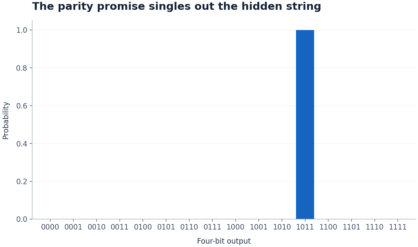
The parity promise singles out the hidden string
Inputs: Display all sixteen four-bit outputs for the fixed parity mask s=1011 and the ideal Bernstein–Vazirani oracle.
P(y=s)=1; P(y≠s)=0 under the exact parity promise.
Calculated results under the declared teaching model
Decoded integer (four-bit output)
Ideal output
0
0
1
0
3
0
5
0
7
0
9
0
11
1
13
0
15
0
The algorithm’s compactness comes from the promise: all responses follow one linear parity rule. Removing that structure changes the problem. The reader should see the cancellation explicitly rather than accept “quantum parallelism” as a complete explanation. A four-bit case is small enough to enumerate every input and verify every sign.
A distinction to keep
The tempting conclusion: A familiar-looking probability or resource count establishes the broader claim without checking its model.
What follows instead: One oracle call is not one ordinary processor instruction and does not include the engineering cost of supplying the promised oracle.
Can the algorithm reveal any hidden database?
No. The oracle must implement the stated parity structure. An arbitrary lookup table has a different problem definition and access cost.
Why do the other answers vanish?
Their signed contributions pair off with opposite phases in the final transform. The cancellation follows from the promised parity function.
Does a noisy device still return one string every time?
Each shot returns a string, but real output frequencies can spread. The teaching calculation describes the ideal distribution and must be labelled separately from hardware results.
For candidate y=1001 and secret s=1011, identify a bit position that makes the phase sum cancel.
The strings differ in the third position when written left to right. Pair each x with the x obtained by flipping that position. Their exponents differ by one, so their contributions have opposite signs. All sixteen terms cancel in eight pairs.
Primary scientific context for an original ideal teaching example. Source research checked 19 October 2026; site integration inspected 20 October 2026. These are different checks.
Mechanism guideThe promise is part of the quantum algorithmWhy does Deutsch-Jozsa need to know which functions are allowed?
Source research checked . Teaching calculations are ideal models.
An algorithm can be extraordinarily effective when the possible inputs belong to a carefully defined family. Deutsch-Jozsa is a classic example. The unknown Boolean function is promised to be either constant or balanced, with exactly half its outputs equal to each value. An ideal quantum procedure distinguishes those two cases with one coherent query. Remove the promise and the interpretation changes. This is not an obscure qualification. It is a direct lesson in how a problem definition can create the conditions for an algorithmic advantage. A reader who understands the promise can judge a far wider range of computational claims.
The phase oracle assigns a plus or minus sign to each input according to the function value. After the final Hadamards, the amplitude of the all-zero output is the average of those signs. A constant function gives an average of plus one or minus one and therefore an all-zero outcome with probability one. A balanced function gives an average of zero and never produces all zeros in the ideal model. A function outside those two families generally gives an intermediate probability. The circuit still runs, but its output is no longer the promised yes-or-no certification. A procedure and the theorem describing its answer must therefore be kept together.
Compare three sign patterns: all signs equal, an even split, and an unpromised split. The first two yield the exact verdicts of the promised problem. The third can produce a nonzero but nonunit all-zero probability, revealing why the promise is a mathematical input. Exact deterministic classical query comparisons and bounded-error randomized classical strategies are different benchmarks. The allowed error probability and access model change the scale of the claimed separation, so both belong beside a query-cost comparison.
The Deutsch-Jozsa decision rule is exact for the promised alternatives. A function is constant or balanced. Once that condition is removed, the same circuit can still be run, but its outcome no longer carries the original guaranteed classification. This is a useful pattern far beyond one textbook algorithm: an algorithm's promise is part of its input specification.
Imagine applying the circuit to a dataset whose labels are only approximately balanced. A zero-string outcome does not license a claim that the function is constant, and the absence of that outcome does not repair the missing promise. A careful report would state the actual label distribution and interpret the resulting probability under a broader model. It would also compare classical and quantum access on the same problem. The best use of the small example is to show where an exact theorem ends and a different statistical inference task begins.
Synthetic worked example
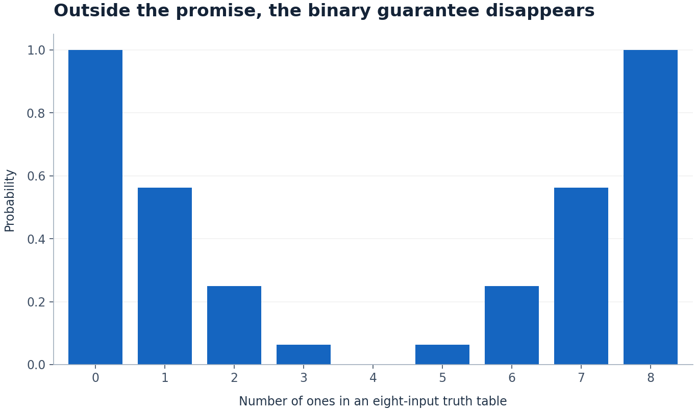
Outside the promise, the binary guarantee disappears
Inputs: Sweep k, the number of ones in an eight-input Boolean truth table, from 0 to 8. Values outside k=0,4,8 illustrate violation of the Deutsch–Jozsa promise.
P(all-zero output)=(1−2k/8)².
Calculated results under the declared teaching model
Number of ones in an eight-input truth table
All-zero output
0
1
1
0.5625
2
0.25
3
0.0625
4
0
5
0.0625
6
0.25
7
0.5625
8
1
A valid theorem can coexist with unhelpful output on an invalid input. That is why benchmark descriptions must include promised structure and preprocessing. In this toy example the violation is visible by enumerating eight values. In a large application, verifying the promise may itself have a cost, and that cost belongs in any end-to-end argument.
A distinction to keep
The tempting conclusion: A familiar-looking probability or resource count establishes the broader claim without checking its model.
What follows instead: An output outside the promised case is not evidence that quantum mechanics has failed. It may simply mean the algorithm was asked a different question.
Does an algorithm stop working outside its promise?
Its circuit can still execute. The theorem guaranteeing a particular interpretation may no longer apply, which is a different statement from an execution failure.
Why compare amplitudes before probabilities?
Interference combines signed or complex amplitudes. Adding probabilities too early removes the cancellation that the algorithm uses.
Is every classical comparison exponential?
No. The comparison depends on the allowed error and query strategy. The article must state the exact model instead of borrowing a dramatic bound from a different setting.
For a truth table with seven zeros and one one, find the all-zero probability. Can the all-zero outcome certify constancy for arbitrary functions?
The amplitude is (7-1)/8=3/4 and the probability is 9/16. A nonconstant function can therefore produce that outcome. The certainty statement requires the original constant-or-balanced promise.
Primary scientific context for an original ideal teaching example. Source research checked 19 October 2026; site integration inspected 20 October 2026. These are different checks.
Mechanism guideClose quantum states need a ruler with a nameWhy do fidelity and trace distance answer different questions?
Source research checked . Teaching calculations are ideal models.
A claim that a quantum state is close to a target leaves a practical question unanswered: close according to which ruler? Different mathematical measures emphasize different operational tasks. Fidelity describes overlap in a widely used family of conventions. Trace distance connects directly to how distinguishable two states can be by measurement. They are related, but a value copied from one definition cannot simply be pasted into the other. Even fidelity itself appears both squared and unsquared in legitimate sources. A good article identifies the convention before comparing numbers.
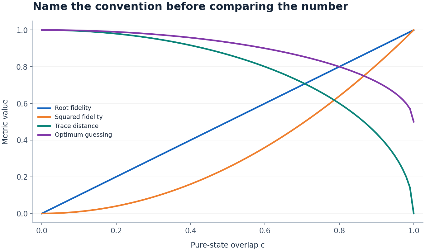
For two pure states with overlap magnitude c, root fidelity is c, squared fidelity is c squared and trace distance is the square root of one minus c squared. Choose c=0.8 and the same pair of states has three different-looking values: 0.8, 0.64 and 0.6. None is an error. Each labels a different quantity. In the equal-prior discrimination task, the optimal chance of distinguishing the states is one half times one plus their trace distance. The example therefore connects the ruler to a question a reader can understand: how well could the best allowed measurement tell these preparations apart?
A company release, a paper and a dashboard may use the word fidelity in different ways. The number needs its definition, object and protocol. State fidelity, process fidelity and an empirical circuit-success fraction are not interchangeable labels, and source-specific conventions matter. A component measure cannot be converted into the success probability of a long application without a justified error model. Keeping the operational meaning attached makes the value more informative.
Two technical documents can report different-looking percentages for the same underlying overlap because one uses root fidelity and the other uses its square. For example, a root value of 0.9 corresponds to a squared value of 0.81. Reading those numbers as if they shared a definition would create a performance difference that the mathematics does not contain.
Before placing reported metrics in a comparison table, copy their actual definitions and identify the states, channels or operations being compared. Preserve uncertainty and any conditioning or postselection in the original measurement. A state-fidelity convention also should not be substituted for a gate-error rate merely because both appear as percentages. The small worked example supplies a clean place to learn the convention change. Its trace distance and discrimination interpretation are separate quantities with their own definitions. A useful comparison makes the mathematical object and denominator visible before readers react to the number of nines.
Synthetic worked example
Name the convention before comparing the number
Inputs: Sweep pure-state overlap magnitude c from 0 to 1. Equal priors apply only to the optimum-guessing comparison.
Calculated results under the declared teaching model
Pure-state overlap c
Root fidelity
Squared fidelity
Trace distance
Optimum guessing
0
0
0
1
1
0.12
0.12
0.0144
0.9927738916792685
0.9963869458396343
0.25
0.25
0.0625
0.9682458365518543
0.9841229182759271
0.37
0.37
0.1369
0.9290317540321213
0.9645158770160607
0.5
0.5
0.25
0.8660254037844386
0.9330127018922193
0.62
0.62
0.3844
0.7846018098373212
0.8923009049186605
0.75
0.75
0.5625
0.6614378277661477
0.8307189138830738
0.87
0.87
0.7569
0.493051721424842
0.746525860712421
1
1
1
0
0.5
A metric name without its mathematical convention is an incomplete data field. The same states can legitimately produce different numbers called fidelity in different sources. This does not make comparisons impossible; it makes normalization necessary. A table containing definition, state class, denominator and confidence interval is often more useful than a ranked list of percentages.
A distinction to keep
The tempting conclusion: A familiar-looking probability or resource count establishes the broader claim without checking its model.
What follows instead: The pure-state equality between overlap and trace distance does not extend unchanged to arbitrary mixed states. Use appropriate inequalities or calculate the matrix quantities.
Which fidelity convention is correct?
Both squared and root conventions are used. The source definition must be retained consistently; the convention is not settled by choosing the more impressive percentage.
Does high state fidelity prove useful speedup?
No. It describes a state comparison. A speedup claim requires a task, required output quality and a complete competing workflow.
Can the values be compared across systems?
Only after matching the measured object, definition, protocol, conditions and uncertainty. Identical labels can still conceal different experiments.
Find the overlap for which root fidelity equals the equal-prior optimum guessing probability. Is c=0.8 a general identity?
Solve c=(1+√(1-c²))/2 with c≥1/2. Squaring gives 5c²-4c=0, so the valid solution is c=0.8. It is a special crossing point, not an equality between the definitions for all states.
Primary scientific context for an original ideal teaching example. Source research checked 19 October 2026; site integration inspected 20 October 2026. These are different checks.
Primary scientific context for an original ideal teaching example. Source research checked 19 October 2026; site integration inspected 20 October 2026. These are different checks.
Mechanism guideThe quantum game whose rules make the surprise testableWhy does the CHSH game have different classical and quantum success limits?
Source research checked . Teaching calculations are ideal models.
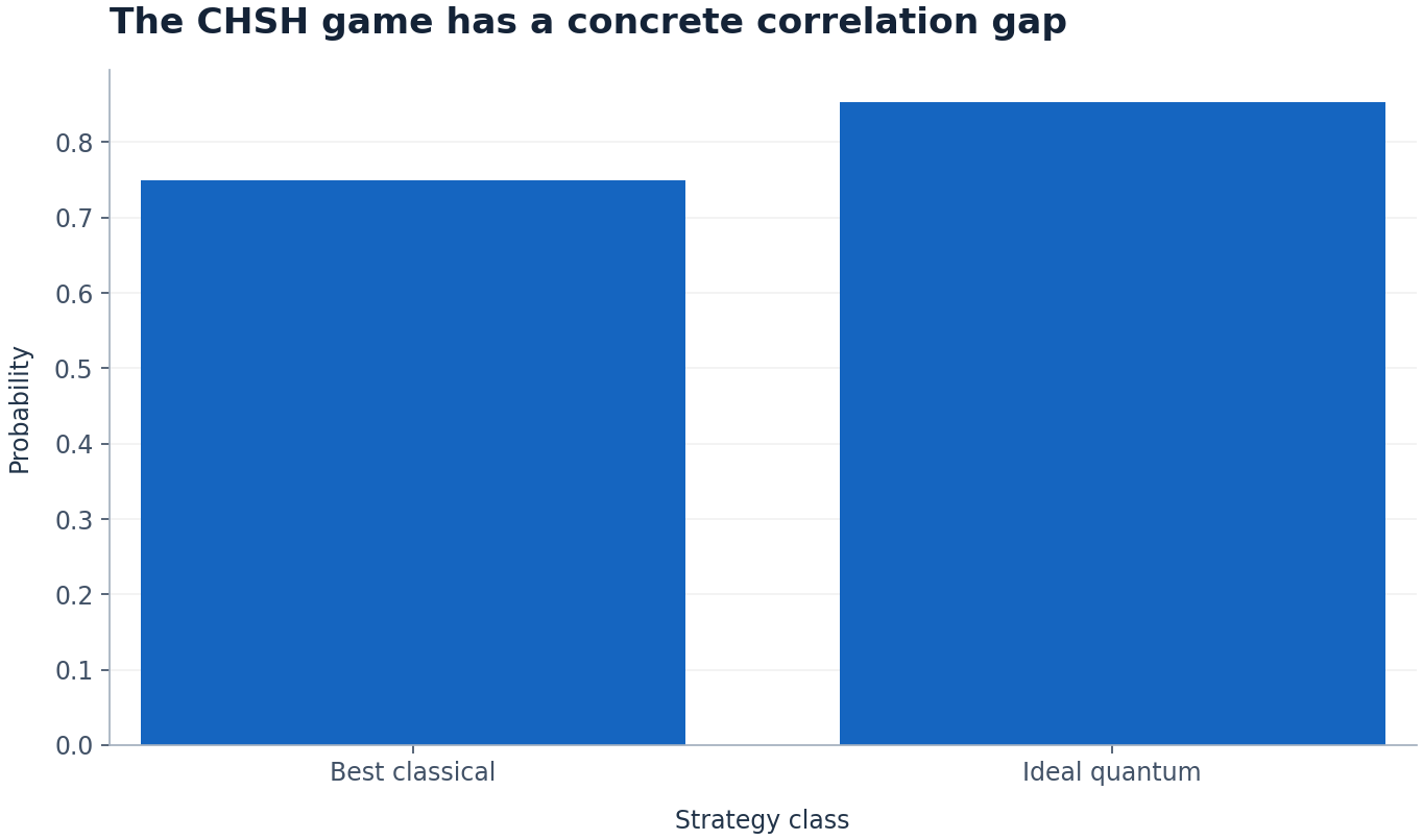
Two players receive separate random input bits and must return output bits without communicating after the inputs arrive. They win if the parity of their answers equals the product of the input bits. The rule is simple enough to check on four cards. With classical shared randomness they can win at most three quarters of the trials under the game assumptions. With an appropriate shared entangled state and local measurements, quantum theory allows a larger success probability. The surprise is compelling because the conditions and the scoring rule can be made explicit before the result is shown.
For a fixed classical strategy, each player chooses a response to each possible local input. The four required parity equations cannot all hold at once: adding the first three modulo two conflicts with the fourth. A deterministic strategy can satisfy three, and mixing deterministic strategies with shared randomness cannot improve the average bound when inputs are uniform and independent. The ideal quantum strategy changes the allowed correlations rather than sending a last-second message. Its success probability is cos squared of pi over eight, about 0.853553. A real Bell experiment needs additional care about separation, detection, input generation and statistical evidence before drawing its physical conclusion.
Try assigning the four classical responses, one for each player's possible local input. The parity obstruction appears before the quantum prediction is introduced, with the no-communication rule unchanged. A precise inequality can connect measured correlations to conclusions about randomness or network entanglement under explicit assumptions. A same-chip educational demonstration and a loophole-free spacelike-separated Bell experiment provide different forms of physical evidence even when they illustrate related mathematics.
A CHSH winning percentage is meaningful only with a defined input distribution and communication rule. Under the game in this example, the four input pairs are equally likely and the players cannot exchange information after their questions arrive. The classical and quantum comparisons are derived for those conditions.
A laboratory test adds questions about how settings and outcomes were generated, which trials were included and how statistical uncertainty was handled. The ideal score does not answer those experimental questions automatically. A commercial performance benchmark is a further distinct claim and needs its own task and resources. This makes CHSH a strong introductory example of both quantum correlations and disciplined comparison. Ask first whether the observed statistic corresponds to the stated game. Then ask whether the evidence supports the intended inference. Keeping those layers separate explains the significance of the ideal advantage without implying faster-than-light communication or an unrestricted computational speedup.
Synthetic worked example
The CHSH game has a concrete correlation gap
Inputs: Compare the best classical and ideal quantum CHSH strategies with uniform independent inputs and no communication after inputs.
Calculated results under the declared teaching model
Strategy class
Win probability
Best classical
0.75
Ideal quantum
0.8535533905932737
The game converts an abstract inequality into a score with a clear denominator. The quantum advantage concerns correlations under restricted communication, not faster-than-light messaging. Changing the input distribution or allowing communication changes the comparison, so the rules belong beside the score.
A distinction to keep
The tempting conclusion: A familiar-looking probability or resource count establishes the broader claim without checking its model.
What follows instead: A violation of a local classical correlation bound does not let either player choose the other player’s local outcome to send a message.
Can shared randomness beat the bound?
Not under the stated uniform-input no-communication game. Shared randomness mixes deterministic strategies, each of which obeys the same maximum average score.
Does the game send a message?
No. The parties cannot use the correlations to communicate their new inputs without a channel. The advantage appears when the records are later compared.
Is every chip demonstration loophole-free?
No. An instructional circuit and a separated Bell test have different experimental conditions. Report the actual geometry, input generation and detection assumptions.
Choose the always-zero classical strategy. Which input pair loses, and what score results? Why can randomizing several such strategies not beat the best deterministic score?
The pair x=y=1 requires opposite outputs and therefore loses. The other three pairs win. A shared-randomness strategy is a probability-weighted average of deterministic scores, so it cannot exceed their maximum.
The animated bar fill reveals static ideal-model values; it is not a measured time series. Uniform inputs; no communication after the questions arrive.
Read the complete transcript
A game with a quantum edge
00–08 seconds
Two players get separate random bits
Each returns one bit. They cannot communicate after receiving the questions.
08–16 seconds
There are four equally likely inputs
They win when the XOR of their answers equals the AND of the two input bits.
16–24 seconds
Classical strategies reach 75%
A deterministic strategy can satisfy three of the four cases. Shared randomness cannot improve the maximum.
24–32 seconds
An entangled strategy reaches 85.36%
The ideal quantum strategy gives cos squared(pi/8), about 0.853553.
32–40 seconds
The rules are part of the result
Uniform inputs and no communication are essential. Laboratory loopholes and finite statistics need evidence.
40–48 seconds
Correlations do not send messages
Explore the worked CHSH game. The advantage does not allow faster-than-light communication.
All typography, charts, geometry, animation and captions are original Volume IX work. No external footage, music or photographs are incorporated. Production checked .
Primary scientific context for an original ideal teaching example. Source research checked 19 October 2026; site integration inspected 20 October 2026. These are different checks.
Evidence and experimental designA better result in every workload can lose the combined scoreCan a changing workload mix reverse a performance comparison?
Source research checked . Teaching calculations are ideal models.
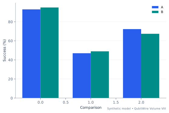
A benchmark suite is a distribution of questions. If a provider runs mostly easy instances while another tackles mostly hard ones, their overall completion percentages answer different questions. Neither percentage is wrong as a description of its own workload. The mistake occurs when the two denominators are treated as interchangeable evidence about the methods.
The constructed example contains only two strata, easy and hard. Method B improves the stipulated success probability in both. It is nevertheless possible to make B look worse overall by allocating more hard work to B. The reversal comes entirely from the weights. There is no hidden quantum effect and no arithmetic paradox once those weights become visible.
Standardization chooses one reference workload and evaluates both methods against it. That requires a defensible reference: the published challenge set, a fixed deployment distribution or a clearly labeled teaching mixture. A fair comparison keeps both the observed mix and the standardized comparison. Discarding the operational mix can erase useful information about what a service actually handled; discarding standardization can reward an easier test.
Synthetic decision model
Start with the assumptions
Within-stratum rates are known synthetic probabilities.
Easy and hard are fixed categories with comparable meanings.
No uncertainty intervals are attached to stipulated rates.
Standardized success uses the same easy_fraction for both methods
Percentage-point difference = 100 × (p_B - p_A)
Synthetic baseline case. Horizontal axis: Comparison. Vertical axis: Success (%). Curves show A, B. These are computed teaching examples, not measured hardware results.
Compare the input regimes
Each case uses invented inputs. The results follow from this model and do not describe measured hardware.
Baseline regime
Complete inputs
A easy success
0.93
A hard success
0.47
B within-stratum gain
0.02
A easy workload fraction
0.55
B easy workload fraction
0.4
Reference easy fraction
0.2
A is weighted using 55% easy work; B uses 40%. Those are different test distributions.
Use the shared 20% easy reference for both: A = 0.562, B = 0.582.
The raw difference is -4.9 percentage points. The shared-workload difference is 2 percentage points.
Baseline regime · synthetic calculated results
Calculated quantity
Synthetic result
A mixed success (%)
72.30000000000001
B mixed success (%)
67.4
Raw B minus A (percentage points)
-4.900000000000004
A standardized success (%)
56.2
B standardized success (%)
58.20000000000001
Standardized gain (percentage points)
2.0000000000000018
The direction reverses after standardization. B was defined to improve both strata by 2 percentage points. Aggregation cannot identify that fact without the workload mix. These rates are stipulated probabilities, not estimates with sampling intervals.
Comparison regime
Complete inputs
A easy success
0.93
A hard success
0.47
B within-stratum gain
0.03
A easy workload fraction
0.7000000000000001
B easy workload fraction
0.325
Reference easy fraction
0.45
A is weighted using 70% easy work; B uses 32.5%. Those are different test distributions.
Use the shared 45% easy reference for both: A = 0.677, B = 0.707.
The raw difference is -14.25 percentage points. The shared-workload difference is 3 percentage points.
Comparison regime · synthetic calculated results
Calculated quantity
Synthetic result
A mixed success (%)
79.2
B mixed success (%)
64.95
Raw B minus A (percentage points)
-14.249999999999996
A standardized success (%)
67.7
B standardized success (%)
70.7
Standardized gain (percentage points)
3.0000000000000027
The direction reverses after standardization. B was defined to improve both strata by 3 percentage points. Aggregation cannot identify that fact without the workload mix. These rates are stipulated probabilities, not estimates with sampling intervals.
Extended regime
Complete inputs
A easy success
0.93
A hard success
0.47
B within-stratum gain
0.041999999999999996
A easy workload fraction
0.88
B easy workload fraction
0.23500000000000004
Reference easy fraction
0.75
A is weighted using 88% easy work; B uses 23.5%. Those are different test distributions.
Use the shared 75% easy reference for both: A = 0.815, B = 0.857.
The raw difference is -25.47 percentage points. The shared-workload difference is 4.2 percentage points.
Extended regime · synthetic calculated results
Calculated quantity
Synthetic result
A mixed success (%)
87.48
B mixed success (%)
62.01000000000001
Raw B minus A (percentage points)
-25.46999999999999
A standardized success (%)
81.5
B standardized success (%)
85.7
Standardized gain (percentage points)
4.200000000000015
The direction reverses after standardization. B was defined to improve both strata by 4.2 percentage points. Aggregation cannot identify that fact without the workload mix. These rates are stipulated probabilities, not estimates with sampling intervals.
Try the reasoning: Choose a second common workload distribution. Does the within-stratum improvement change, or only the aggregate score?
Algorithms and useful workThe best answer depends on how many complete attempts fitWhich solver gives the best result before one fixed deadline?
Source research checked . Teaching calculations are ideal models.
A fast solver can make many modest attempts while a slower solver spends more effort on each attempt. Comparing only their best single-run success probabilities ignores that operational difference. Comparing only runtime ignores the quality distribution. A fixed wall-clock deadline gives the two quantities a common setting.
The constructed strategies return one of three quality levels with known probabilities. The distribution of the best answer after repeated independent runs follows from the probability that every answer stays below a threshold. That gives both the chance of reaching top quality and the expected best score. These are related but distinct summaries of the same campaign.
The lab includes a one-time setup cost before counting complete runs. It does not grant either strategy free tuning or changing instances. The cases can enrich an optimization guide by showing how a quality-versus-time claim should be framed. A real benchmark would need actual distributions from matched instances, confidence intervals and a clear policy for incomplete runs. The synthetic result supplies a comparison design, not evidence for a quantum solver advantage.
Synthetic decision model
Start with the assumptions
Runs are independent and their distributions do not change.
Both strategies use the same quality scale and fixed problem.
Incomplete runs return no usable answer.
Completed runs = floor((deadline-setup)/time per run), with minimum zero
Expected best quality is a sum of quality increments times exceedance probabilities
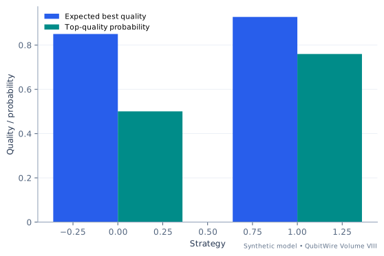
Synthetic baseline case. Horizontal axis: Strategy. Vertical axis: Quality / probability. Curves show Expected best quality, Top-quality probability. These are computed teaching examples, not measured hardware results.
Compare the input regimes
Each case uses invented inputs. The results follow from this model and do not describe measured hardware.
Baseline regime
Complete inputs
Time budget, seconds
80
Setup per strategy, seconds
10
A seconds per run
4
B seconds per run
15
A high-quality probability
0.04
B high-quality probability
0.3
Quality levels
0.4, 0.7, 1
A fraction of non-top outcomes at lowest quality
0.55
B fraction of non-top outcomes at lowest quality
0.3
Subtract setup before counting complete runs: A fits 17; B fits 4. An unfinished run contributes no result.
For independent repeats, the probability all answers lie below a quality level is the single-run cumulative probability raised to the number of runs. This gives the distribution of the best answer.
The top-quality probabilities are 0.500413 and 0.7599. Summing the quality-level increments times their exceedance probabilities gives expected best values 0.850118 and 0.927387.
Baseline regime · synthetic calculated results
Calculated quantity
Synthetic result
Completed A runs
17
Completed B runs
4
A probability of top-quality answer
0.5004131923201862
B probability of top-quality answer
0.7599
A expected best quality
0.8501181780939879
B expected best quality
0.927386557
Complete single-run quality distributions
Quality
A probability
B probability
0.4
0.528
0.21
0.7
0.432
0.48999999999999994
1
0.04
0.3
B has the higher expected best quality under the declared deadline. The quality scale, distributions and runtimes are invented. This comparison is meaningful only if both methods solve the same fixed instance and use the same scoring rule; repeated attempts must not silently receive new tuning information.
Comparison regime
Complete inputs
Time budget, seconds
180
Setup per strategy, seconds
20
A seconds per run
6
B seconds per run
20
A high-quality probability
0.07
B high-quality probability
0.4
Quality levels
0.4, 0.7, 1
A fraction of non-top outcomes at lowest quality
0.55
B fraction of non-top outcomes at lowest quality
0.3
Subtract setup before counting complete runs: A fits 26; B fits 8. An unfinished run contributes no result.
For independent repeats, the probability all answers lie below a quality level is the single-run cumulative probability raised to the number of runs. This gives the distribution of the best answer.
The top-quality probabilities are 0.84845 and 0.983204. Summing the quality-level increments times their exceedance probabilities gives expected best values 0.954535 and 0.994961.
Comparison regime · synthetic calculated results
Calculated quantity
Synthetic result
Completed A runs
26
Completed B runs
8
A probability of top-quality answer
0.8484497481581527
B probability of top-quality answer
0.98320384
A expected best quality
0.9545349163730907
B expected best quality
0.9949608214011828
Complete single-run quality distributions
Quality
A probability
B probability
0.4
0.5115
0.18
0.7
0.4185
0.42
1
0.07
0.4
B has the higher expected best quality under the declared deadline. The quality scale, distributions and runtimes are invented. This comparison is meaningful only if both methods solve the same fixed instance and use the same scoring rule; repeated attempts must not silently receive new tuning information.
Extended regime
Complete inputs
Time budget, seconds
300
Setup per strategy, seconds
32
A seconds per run
6
B seconds per run
26
A high-quality probability
0.10600000000000001
B high-quality probability
0.52
Quality levels
0.4, 0.7, 1
A fraction of non-top outcomes at lowest quality
0.55
B fraction of non-top outcomes at lowest quality
0.3
Subtract setup before counting complete runs: A fits 44; B fits 10. An unfinished run contributes no result.
For independent repeats, the probability all answers lie below a quality level is the single-run cumulative probability raised to the number of runs. This gives the distribution of the best answer.
The top-quality probabilities are 0.992775 and 0.999351. Summing the quality-level increments times their exceedance probabilities gives expected best values 0.997832 and 0.999805.
Extended regime · synthetic calculated results
Calculated quantity
Synthetic result
Completed A runs
44
Completed B runs
10
A probability of top-quality answer
0.9927747841325296
B probability of top-quality answer
0.9993507493789145
A expected best quality
0.9978324352397507
B expected best quality
0.9998052236635464
Complete single-run quality distributions
Quality
A probability
B probability
0.4
0.4917
0.144
0.7
0.4023
0.33599999999999997
1
0.10600000000000001
0.52
B has the higher expected best quality under the declared deadline. The quality scale, distributions and runtimes are invented. This comparison is meaningful only if both methods solve the same fixed instance and use the same scoring rule; repeated attempts must not silently receive new tuning information.
Try the reasoning: Which strategy maximizes the expected best score, and which maximizes top-quality probability? Would a different deadline change the choice?
Algorithms and useful workThe most likely single quantum search is not always the best campaignHow should an ideal search trade amplification depth for additional attempts?
Source research checked . Teaching calculations are ideal models.
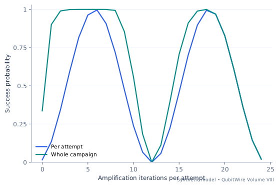
Amplitude amplification rotates an ideal state toward a marked subspace, but continuing the rotation can move it away again. A familiar teaching problem asks how many iterations maximize the success of one attempt. A complete workflow can ask a different question: how many iterations leave the best overall chance of success within one time budget?
The lab uses the ideal two-dimensional rotation formula and adds an explicit preparation cost and oracle-equivalent timing convention. Each candidate depth allows a different number of complete restarts. The campaign success is then calculated from those independent attempts. The best single attempt and best whole campaign are reported separately rather than forcing them into one headline ratio.
This is an extension of an algorithm lesson, not a practical speedup estimate. A real oracle must be constructed and uncomputed, data preparation must be counted, and marked outputs need verification. Those costs can dominate an application. The useful interaction lets the reader increase preparation cost while leaving the ideal quantum rotation unchanged, making clear that algorithmic probability and complete workload time are separate layers of evidence.
Synthetic decision model
Start with the assumptions
The ideal amplitude-amplification model is exact in the synthetic calculation.
The timing convention is chosen for this exercise.
Restarts are independent and verification is included only through the declared budget convention.
theta = asin(sqrt(marked fraction))
Ideal per-attempt success = sin²((2k+1)theta)
Declared attempt time = preparation + (2k+1) × oracle-equivalent time
Synthetic baseline case. Horizontal axis: Amplification iterations per attempt. Vertical axis: Success probability. Curves show Per attempt, Whole campaign. These are computed teaching examples, not measured hardware results.
Compare the input regimes
Each case uses invented inputs. The results follow from this model and do not describe measured hardware.
Baseline regime
Complete inputs
Marked fraction
0.015625
Oracle-equivalent time
1
Preparation time
2
Total time budget
80
Maximum iterations per attempt
24
The ideal success after k iterations is sin²((2k+1)theta), where theta = asin(sqrt(0.015625)).
The declared attempt time is preparation + (2k+1) × oracle-equivalent time. The factor 2k+1 is this exercise’s accounting convention, not a universal decomposition of a Grover circuit.
At k = 6, 5 complete independent attempts fit. Their combined success is 1-(1-p)^attempts = 1.
Baseline regime · synthetic calculated results
Calculated quantity
Synthetic result
Best tested iterations per attempt
6
Attempts fitting the budget
5
Success per chosen attempt
0.9965856807867991
Campaign success probability
0.999999999999536
Best single-attempt iteration count
6
Unamplified campaign success
0.3359894766227789
Unamplified attempt and the two distinct optimization objectives
Iterations
Single-attempt success
Duration
Complete attempts
Campaign success
0
0.015625
3
26
0.3359894766227789
6
0.9965856807867991
15
5
0.999999999999536
The best tested campaign choice is k = 6; the best single-attempt probability occurs at k = 6. They optimize different quantities. A real advantage claim must also establish the oracle construction, state preparation, verification and fair classical search cost; this ideal rotation model supplies none of those performance facts.
Comparison regime
Complete inputs
Marked fraction
0.004464285714285714
Oracle-equivalent time
1.5
Preparation time
27
Total time budget
180
Maximum iterations per attempt
24
The ideal success after k iterations is sin²((2k+1)theta), where theta = asin(sqrt(0.004464)).
The declared attempt time is preparation + (2k+1) × oracle-equivalent time. The factor 2k+1 is this exercise’s accounting convention, not a universal decomposition of a Grover circuit.
At k = 11, 2 complete independent attempts fit. Their combined success is 1-(1-p)^attempts = 0.999999.
Comparison regime · synthetic calculated results
Calculated quantity
Synthetic result
Best tested iterations per attempt
11
Attempts fitting the budget
2
Success per chosen attempt
0.9989180813519019
Campaign success probability
0.9999988294520389
Best single-attempt iteration count
11
Unamplified campaign success
0.026488540084901542
Unamplified attempt and the two distinct optimization objectives
Iterations
Single-attempt success
Duration
Complete attempts
Campaign success
0
0.004464285714285715
28.5
6
0.026488540084901542
11
0.9989180813519019
61.5
2
0.9999988294520389
The best tested campaign choice is k = 11; the best single-attempt probability occurs at k = 11. They optimize different quantities. A real advantage claim must also establish the oracle construction, state preparation, verification and fair classical search cost; this ideal rotation model supplies none of those performance facts.
Extended regime
Complete inputs
Marked fraction
0.002403846153846154
Oracle-equivalent time
2.1
Preparation time
57
Total time budget
300
Maximum iterations per attempt
24
The ideal success after k iterations is sin²((2k+1)theta), where theta = asin(sqrt(0.002404)).
The declared attempt time is preparation + (2k+1) × oracle-equivalent time. The factor 2k+1 is this exercise’s accounting convention, not a universal decomposition of a Grover circuit.
At k = 16, 2 complete independent attempts fit. Their combined success is 1-(1-p)^attempts = 0.999995.
Extended regime · synthetic calculated results
Calculated quantity
Synthetic result
Best tested iterations per attempt
16
Attempts fitting the budget
2
Success per chosen attempt
0.9977158771365623
Campaign success probability
0.9999947827827447
Best single-attempt iteration count
16
Unamplified campaign success
0.011961584744724526
Unamplified attempt and the two distinct optimization objectives
Iterations
Single-attempt success
Duration
Complete attempts
Campaign success
0
0.002403846153846154
59.1
5
0.011961584744724526
16
0.9977158771365623
126.3
2
0.9999947827827447
The best tested campaign choice is k = 16; the best single-attempt probability occurs at k = 16. They optimize different quantities. A real advantage claim must also establish the oracle construction, state preparation, verification and fair classical search cost; this ideal rotation model supplies none of those performance facts.
Try the reasoning: Compare the campaign optimum with the single-attempt optimum. Which preparation and restart costs make their objectives differ?
Ideal amplitude amplification rotates a state in a two-dimensional subspace and can overshoot the desired marked population. The lab's timing convention and campaign budget are independently chosen; no hardware runtime, API version or practical advantage is claimed.
Quantum information foundationsThe hidden string appears through a promised oracleWhat makes Bernstein-Vazirani an instructive speedup without making it a universal search engine?
Source research checked . Teaching calculations are ideal models.
The oracle computes the parity of a secret bit string s with an input x. Choose s=1011 and four input bits. The task is to identify s through calls to this specified oracle. It is not a model of opening arbitrary files or searching a database without accounting for how the oracle is built.
The algorithm’s compactness comes from the promise: all responses follow one linear parity rule. Removing that structure changes the problem. The reader should see the cancellation explicitly rather than accept “quantum parallelism” as a complete explanation. A four-bit case is small enough to enumerate every input and verify every sign.
Figure and table scope: Display all sixteen four-bit outputs for the fixed parity mask s=1011 and the ideal Bernstein–Vazirani oracle.
Derivation step 1: Prepare the input register in an equal superposition of every x and an auxiliary target in minus. The oracle’s output flip becomes a phase (-1)^(s·x).
Derivation step 2: Apply a Hadamard to every input qubit. The amplitude of a candidate output y is the average of (-1)^((s⊕y)·x) over all x.
Derivation step 3: When y=s, every term equals one. When y differs from s in at least one position, terms pair off with opposite signs and sum to zero.
Derivation step 4: The ideal output is therefore 1011 in the stated register order. Oracle construction and control accuracy are outside this query-count derivation.
Separate challenge: For candidate y=1001 and secret s=1011, identify a bit position that makes the phase sum cancel.
Worked challenge answer: The strings differ in the third position when written left to right. Pair each x with the x obtained by flipping that position. Their exponents differ by one, so their contributions have opposite signs. All sixteen terms cancel in eight pairs.
Synthetic decision model
Start with the assumptions
Exact parity promise, coherent oracle access, no noise and a declared bit order. The count is oracle queries, not a complete end-to-end runtime benchmark.
P(y=s)=1; P(y≠s)=0 under the exact parity promise.
Display all sixteen four-bit outputs for the fixed parity mask s=1011 and the ideal Bernstein–Vazirani oracle. Original ideal teaching calculation. Not measured hardware data.
Compare the input regimes
Each case uses invented inputs. The results follow from this model and do not describe measured hardware.
Reference example with separately scoped figure
Complete inputs
reference scenario
Let s=1011 and f(x)=s dot x modulo two. Compute the ideal final state after Hadamards, a phase oracle and Hadamards.
separate figure scope
Display all sixteen four-bit outputs for the fixed parity mask s=1011 and the ideal Bernstein–Vazirani oracle.
Amplitude of output y = 2^(-n) sum_x (-1)^[(s xor y) dot x]. This equals 1 for y=s and 0 otherwise.
Reference example with separately scoped figure · synthetic calculated results
Reference
Prediction
Original declared example
For four input qubits the output is 1011 with certainty in the ideal promised setting. Classical single-position queries return the four mask bits separately.
Separate figure table: Display all sixteen four-bit outputs for the fixed parity mask s=1011 and the ideal Bernstein–Vazirani oracle.
Decoded integer (four-bit output)
Ideal output
0
0
1
0
3
0
5
0
7
0
9
0
11
1
13
0
15
0
The declared reference example predicts: For four input qubits the output is 1011 with certainty in the ideal promised setting. Classical single-position queries return the four mask bits separately.
Try the reasoning: For candidate y=1001 and secret s=1011, identify a bit position that makes the phase sum cancel.
Primary scientific context for an original ideal teaching example. Source research checked 19 October 2026; site integration inspected 20 October 2026. These are different checks.
Quantum information foundationsWhat happens when an algorithm’s promise is brokenWhy does Deutsch-Jozsa need to know which functions are allowed?
Source research checked . Teaching calculations are ideal models.
Use a three-bit Boolean oracle, so there are eight possible inputs. The Deutsch–Jozsa promise says the function is constant or balanced. The experiment deliberately includes a third case with six zeros and two ones to show why an algorithm’s guarantee depends on its input conditions.
A valid theorem can coexist with unhelpful output on an invalid input. That is why benchmark descriptions must include promised structure and preprocessing. In this toy example the violation is visible by enumerating eight values. In a large application, verifying the promise may itself have a cost, and that cost belongs in any end-to-end argument.
Figure and table scope: Sweep k, the number of ones in an eight-input Boolean truth table, from 0 to 8. Values outside k=0,4,8 illustrate violation of the Deutsch–Jozsa promise.
Derivation step 1: After phase kickback and final Hadamards, the all-zero output amplitude is the average of (-1)^f(x) over all eight inputs.
Derivation step 2: For a constant function this average is either plus one or minus one, so the all-zero output occurs with certainty.
Derivation step 3: For a balanced function four terms are positive and four negative, giving zero all-zero probability.
Derivation step 4: For six zeros and two ones, the average is (6-2)/8=1/2, so the all-zero probability is one quarter. The algorithm’s promised binary interpretation no longer applies.
Separate challenge: For a truth table with seven zeros and one one, find the all-zero probability. Can the all-zero outcome certify constancy for arbitrary functions?
Worked challenge answer: The amplitude is (7-1)/8=3/4 and the probability is 9/16. A nonconstant function can therefore produce that outcome. The certainty statement requires the original constant-or-balanced promise.
Synthetic decision model
Start with the assumptions
Ideal phase oracle and exact counts over all inputs. Query-complexity comparisons must specify deterministic exact versus randomized bounded-error classical strategies.
P(all-zero output)=(1−2k/8)².
Sweep k, the number of ones in an eight-input Boolean truth table, from 0 to 8. Values outside k=0,4,8 illustrate violation of the Deutsch–Jozsa promise. Original ideal teaching calculation. Not measured hardware data.
Compare the input regimes
Each case uses invented inputs. The results follow from this model and do not describe measured hardware.
Reference example with separately scoped figure
Complete inputs
reference scenario
Use three input bits, so the function has eight outputs. Compare constant, four/four balanced and an unpromised six/two split.
separate figure scope
Sweep k, the number of ones in an eight-input Boolean truth table, from 0 to 8. Values outside k=0,4,8 illustrate violation of the Deutsch–Jozsa promise.
Reference example with separately scoped figure · synthetic calculated results
Reference
Prediction
Original declared example
The intermediate case produces all zeros one quarter of the time in the ideal model. It cannot be classified using the promised deterministic rule because it violates the input contract.
Separate figure table: Sweep k, the number of ones in an eight-input Boolean truth table, from 0 to 8. Values outside k=0,4,8 illustrate violation of the Deutsch–Jozsa promise.
Number of ones in an eight-input truth table
All-zero output
0
1
1
0.5625
2
0.25
3
0.0625
4
0
5
0.0625
6
0.25
7
0.5625
8
1
The declared reference example predicts: The intermediate case produces all zeros one quarter of the time in the ideal model. It cannot be classified using the promised deterministic rule because it violates the input contract.
Try the reasoning: For a truth table with seven zeros and one one, find the all-zero probability. Can the all-zero outcome certify constancy for arbitrary functions?
Primary scientific context for an original ideal teaching example. Source research checked 19 October 2026; site integration inspected 20 October 2026. These are different checks.
Quantum information foundationsThree state-comparison numbers from one overlapWhy do fidelity and trace distance answer different questions?
Source research checked . Teaching calculations are ideal models.
Take two pure states with overlap magnitude c=0.8 and equal prior probabilities in a discrimination task. Compute root fidelity, squared fidelity and trace distance, then connect the last quantity to the optimum guessing probability. Restrict the exact equalities to the pure-state case used here.
A metric name without its mathematical convention is an incomplete data field. The same states can legitimately produce different numbers called fidelity in different sources. This does not make comparisons impossible; it makes normalization necessary. A table containing definition, state class, denominator and confidence interval is often more useful than a ranked list of percentages.
Figure and table scope: Sweep pure-state overlap magnitude c from 0 to 1. Equal priors apply only to the optimum-guessing comparison.
Derivation step 1: Root fidelity equals c, so it is 0.8. A convention that squares fidelity reports 0.64 for the same pair.
Derivation step 2: For pure states, trace distance D=√(1-c²), giving 0.6. Here D includes the standard one-half factor in the trace-norm definition.
Derivation step 3: The optimum correct guessing probability for equal priors is (1+D)/2=0.8.
Derivation step 4: A higher similarity measure and a higher distinguishability measure point in opposite directions. The repeated decimal 0.8 in this example has two different definitions and should not be conflated.
Separate challenge: Find the overlap for which root fidelity equals the equal-prior optimum guessing probability. Is c=0.8 a general identity?
Worked challenge answer: Solve c=(1+√(1-c²))/2 with c≥1/2. Squaring gives 5c²-4c=0, so the valid solution is c=0.8. It is a special crossing point, not an equality between the definitions for all states.
Synthetic decision model
Start with the assumptions
Two pure states, equal priors and optimal measurement. Mixed-state relations require the general definitions and cannot be inferred by reusing the pure-state equality.
Sweep pure-state overlap magnitude c from 0 to 1. Equal priors apply only to the optimum-guessing comparison. Original ideal teaching calculation. Not measured hardware data.
Compare the input regimes
Each case uses invented inputs. The results follow from this model and do not describe measured hardware.
Reference example with separately scoped figure
Complete inputs
reference scenario
Use pure states with overlap magnitude c=0.8 and equal prior probabilities.
separate figure scope
Sweep pure-state overlap magnitude c from 0 to 1. Equal priors apply only to the optimum-guessing comparison.
Reference example with separately scoped figure · synthetic calculated results
Reference
Prediction
Original declared example
One state pair yields four valid numbers for four labelled quantities. The best-guess value is a discrimination probability, not the fidelity of a gate or a quantum algorithm.
Separate figure table: Sweep pure-state overlap magnitude c from 0 to 1. Equal priors apply only to the optimum-guessing comparison.
Pure-state overlap c
Root fidelity
Squared fidelity
Trace distance
Optimum guessing
0
0
0
1
1
0.12
0.12
0.0144
0.9927738916792685
0.9963869458396343
0.25
0.25
0.0625
0.9682458365518543
0.9841229182759271
0.37
0.37
0.1369
0.9290317540321213
0.9645158770160607
0.5
0.5
0.25
0.8660254037844386
0.9330127018922193
0.62
0.62
0.3844
0.7846018098373212
0.8923009049186605
0.75
0.75
0.5625
0.6614378277661477
0.8307189138830738
0.87
0.87
0.7569
0.493051721424842
0.746525860712421
1
1
1
0
0.5
The declared reference example predicts: One state pair yields four valid numbers for four labelled quantities. The best-guess value is a discrimination probability, not the fidelity of a gate or a quantum algorithm.
Try the reasoning: Find the overlap for which root fidelity equals the equal-prior optimum guessing probability. Is c=0.8 a general identity?
Primary scientific context for an original ideal teaching example. Source research checked 19 October 2026; site integration inspected 20 October 2026. These are different checks.
Primary scientific context for an original ideal teaching example. Source research checked 19 October 2026; site integration inspected 20 October 2026. These are different checks.
Quantum information foundationsThe CHSH game makes a correlation gap concreteWhy does the CHSH game have different classical and quantum success limits?
Source research checked . Teaching calculations are ideal models.
Two separated players receive independently uniform bits x and y. They return bits a and b and win when a XOR b equals x AND y. They cannot communicate after receiving the inputs. Compare deterministic classical strategies with the ideal quantum strategy under these explicit game rules.
The game converts an abstract inequality into a score with a clear denominator. The quantum advantage concerns correlations under restricted communication, not faster-than-light messaging. Changing the input distribution or allowing communication changes the comparison, so the rules belong beside the score.
Figure and table scope: Compare the best classical and ideal quantum CHSH strategies with uniform independent inputs and no communication after inputs.
Derivation step 1: A deterministic classical strategy assigns outputs a0,a1,b0,b1. There are sixteen possible assignments.
Derivation step 2: Winning all four input pairs would require a0⊕b0=0, a0⊕b1=0, a1⊕b0=0 and a1⊕b1=1. XORing the four left sides gives zero, while the right sides give one, a contradiction.
Derivation step 3: A classical strategy can win three of four input pairs, yielding success probability 3/4 with uniform inputs. Shared randomness cannot exceed the best deterministic average.
Derivation step 4: Appropriate entangled states and measurement settings achieve cos²(π/8), approximately 0.853553, in the ideal quantum model. Experimental demonstrations require their own treatment of loopholes and finite statistics.
Separate challenge: Choose the always-zero classical strategy. Which input pair loses, and what score results? Why can randomizing several such strategies not beat the best deterministic score?
Worked challenge answer: The pair x=y=1 requires opposite outputs and therefore loses. The other three pairs win. A shared-randomness strategy is a probability-weighted average of deterministic scores, so it cannot exceed their maximum.
Synthetic decision model
Start with the assumptions
Uniform independent inputs, no communication after inputs, stated quantum resources and ideal measurements. Experimental significance and loophole closure are separate verification tasks.
Compare the best classical and ideal quantum CHSH strategies with uniform independent inputs and no communication after inputs. Original ideal teaching calculation. Not measured hardware data.
Compare the input regimes
Each case uses invented inputs. The results follow from this model and do not describe measured hardware.
Reference example with separately scoped figure
Complete inputs
reference scenario
Enumerate all deterministic response choices a0,a1,b0,b1, each zero or one. Count wins for the four uniform input pairs.
separate figure scope
Compare the best classical and ideal quantum CHSH strategies with uniform independent inputs and no communication after inputs.
Reference example with separately scoped figure · synthetic calculated results
Reference
Prediction
Original declared example
All 16 deterministic strategies win at most three of the four input cases. The ideal quantum value is about 85.3553%, compared with the 75% classical bound.
Separate figure table: Compare the best classical and ideal quantum CHSH strategies with uniform independent inputs and no communication after inputs.
Strategy class
Win probability
Best classical
0.75
Ideal quantum
0.8535533905932737
The declared reference example predicts: All 16 deterministic strategies win at most three of the four input cases. The ideal quantum value is about 85.3553%, compared with the 75% classical bound.
Try the reasoning: Choose the always-zero classical strategy. Which input pair loses, and what score results? Why can randomizing several such strategies not beat the best deterministic score?
Primary scientific context for an original ideal teaching example. Source research checked 19 October 2026; site integration inspected 20 October 2026. These are different checks.
The experiment improves loading and storage in one apparatus. The atom count and the different cooling tests should not be confused with a processor performance claim.
Hardware · Published · Source report · Sources checked
Its Waterloo research programme will investigate chip-scale magnetless circulators. A delivered component and measured cryogenic performance remain ahead.
Research · Published · Source report · Sources checked
Researchers tested four-dimensional encoding in installed fibre in Concepción. The physical links and a separate detector benchmark answer different questions.
Hardware · Published · Source report · Sources checked
The October announcement describes an operating layer for hybrid computing services. Early access and integration claims remain separate from measured quantum performance.
Business + Policy · Published · Source report · Sources checked
Alexandru Paler, Simon Devitt and Artur Izmaylov also join. Their advisory roles concern scientific direction, with product performance requiring its own evidence.
Research · Published · Source report · Sources checked
Helios improves a logical-memory benchmark and separately tests protected Clifford operations. The statistics and workload define what each rate means.
Combines programmable quantum processors with Qiskit tools, cloud job execution and device calibration records, giving developers a route from circuit design to experiments on hardware.
Provides programmable trapped-ion computers and tools for circuits with mid-circuit measurement, reset and classical feedback, alongside emulators for development.
Traps individual atoms with light and controls their interactions. Aquila programs a physical quantum evolution; Gemini uses gates and atom movement for digital and logical-qubit experiments.
Jay Shah presents quantum-assisted physics-informed neural networks for orbit prediction. A research talk from QuantumGrad’s Qiskit Fall Fest. The presentation is not evidence of operational deployment or quantum advantage. Opens on YouTube.
Chandrika Dutt of Avasant discusses the development of the quantum industry. Strategy opinions and forecasts are the speaker’s views. Opens on YouTube.